Effect of assimilating observation at Fort William
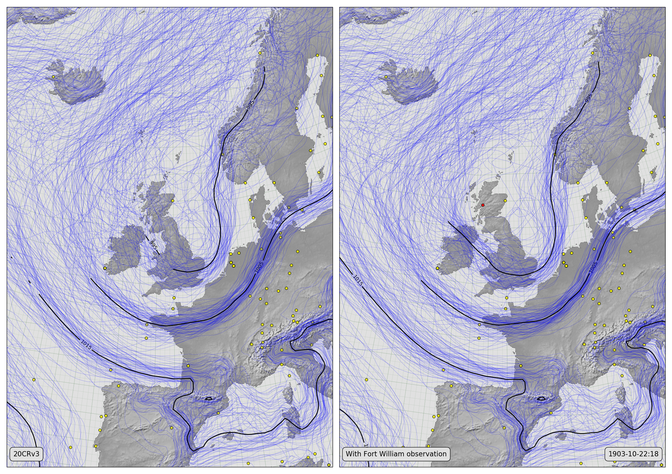
Spaghetti-contour plots showing 20CRv3 MSLP fields before (left) and after (right) assimilating one Fort William observation (October 22nd, 1903 at 6pm).
Code to make the figure
Collect the data (prmsl ensemble and observations from 20CR2c for 1903):
#!/usr/bin/env python

import IRData.twcr as twcr
import datetime
dte=datetime.datetime(1903,10,22)
twcr.fetch('prmsl',dte,version='4.5.1')
twcr.fetch_observations(dte,version='4.5.1')
Script to make the figure:
#!/usr/bin/env python

# Show effect of assimilating single Fort William observation

import math
import datetime
import numpy
import pandas

import iris
import iris.analysis

import matplotlib
from matplotlib.backends.backend_agg import \
             FigureCanvasAgg as FigureCanvas
from matplotlib.figure import Figure

import cartopy
import cartopy.crs as ccrs

import Meteorographica as mg
import IRData.twcr as twcr

import DWR
import DIYA
import sklearn
RANDOM_SEED = 5

# Date to show
year=1903
month=10
day=22
hour=18
dte=datetime.datetime(year,month,day,hour)

# Landscape page
fig=Figure(figsize=(22,22/math.sqrt(2)),  # Width, Height (inches)
           dpi=100,
           facecolor=(0.88,0.88,0.88,1),
           edgecolor=None,
           linewidth=0.0,
           frameon=False,
           subplotpars=None,
           tight_layout=None)
canvas=FigureCanvas(fig)

# UK-centred projection
projection=ccrs.RotatedPole(pole_longitude=177.5, pole_latitude=35.5)
scale=12
extent=[scale*-1,scale,scale*-1*math.sqrt(2),scale*math.sqrt(2)]

# Two side-by-side plots
ax_20C=fig.add_axes([0.01,0.01,0.485,0.98],projection=projection)
ax_20C.set_axis_off()
ax_20C.set_extent(extent, crs=projection)
ax_wFW=fig.add_axes([0.505,0.01,0.485,0.98],projection=projection)
ax_wFW.set_axis_off()
ax_wFW.set_extent(extent, crs=projection)

# Background, grid and land for both
ax_20C.background_patch.set_facecolor((0.88,0.88,0.88,1))
ax_wFW.background_patch.set_facecolor((0.88,0.88,0.88,1))
mg.background.add_grid(ax_20C)
mg.background.add_grid(ax_wFW)
land_img_20C=ax_20C.background_img(name='GreyT', resolution='low')
land_img_DWR=ax_wFW.background_img(name='GreyT', resolution='low')

# 20CR2c data
prmsl=twcr.load('prmsl',dte,version='4.5.1')

# Get the observations used in 20CR2c
obs=twcr.load_observations_fortime(dte,version='4.5.1')
# Filter to those assimilated and near the UK
obs_s=obs.loc[((obs['Latitude']>0) &
                 (obs['Latitude']<90)) &
              ((obs['Longitude']>240) |
                 (obs['Longitude']<100))].copy()
mg.observations.plot(ax_20C,obs_s,radius=0.1)

# For each ensemble member, make a contour plot
CS=mg.pressure.plot(ax_20C,prmsl,
                   resolution=0.25,
                   type='spaghetti',scale=0.01,
                   levels=numpy.arange(875,1050,10),
                   colors='blue',
                   label=False,
                   linewidths=0.2)

# Add the ensemble mean - with labels
prmsl_m=prmsl.collapsed('member', iris.analysis.MEAN)
prmsl_m.data=prmsl_m.data/100 # To hPa
prmsl_s=prmsl.collapsed('member', iris.analysis.STD_DEV)
prmsl_s.data=prmsl_s.data/100
# Mask out mean where uncertainties large
prmsl_m.data[numpy.where(prmsl_s.data>3)]=numpy.nan
CS=mg.pressure.plot(ax_20C,prmsl_m,
                   resolution=0.25,
                   levels=numpy.arange(875,1050,10),
                   colors='black',
                   label=True,
                   linewidths=2)

mg.utils.plot_label(ax_20C,'20CRv3',
                     fontsize=16,
                     facecolor=fig.get_facecolor(),
                     x_fraction=0.02,
                     horizontalalignment='left')

# Get the DWR observations within +- 2 hours
obs=DWR.load_observations('prmsl',
                          dte-datetime.timedelta(hours=2),
                          dte+datetime.timedelta(hours=2))
# Get Fort William value at selected time
fwi=DWR.at_station_and_time(obs,'FORTWILLIAM',dte)
latlon=DWR.get_station_location(obs,'FORTWILLIAM')
obs_assimilate=pandas.DataFrame(data={'year': year,
                                      'month': month,
                                      'day': day,
                                      'hour': hour,
                                      'minute': 0,
                                      'latitude': latlon['latitude'],
                                      'longitude': latlon['longitude'],
                                      'value': fwi*100, #hPa->Pa
                                      'name': 'Fort William'},
                                        index=[0])
obs_assimilate=obs_assimilate.assign(dtm=pandas.to_datetime(
                   obs_assimilate[['year','month',
                                   'day','hour','minute']]))

# Update mslp by assimilating Fort William ob.

prmsl2=DIYA.constrain_cube(prmsl,
                           lambda dte: twcr.load('prmsl',dte,version='4.5.1'),
                           obs=obs_assimilate,
                           obs_error=0.1,
                           random_state=RANDOM_SEED,
                           model=sklearn.linear_model.LinearRegression(),
                           lat_range=(20,85),
                           lon_range=(280,60))

# Plot the assimilated obs
mg.observations.plot(ax_wFW,obs_s,radius=0.1)
# Plot the Fort William ob
mg.observations.plot(ax_wFW,obs_assimilate,lat_label='latitude',
            lon_label='longitude',radius=0.1,facecolor='red')

# For each ensemble member, make a contour plot
CS=mg.pressure.plot(ax_wFW,prmsl2,
                   resolution=0.25,
                   type='spaghetti',scale=0.01,
                   levels=numpy.arange(875,1050,10),
                   colors='blue',
                   label=False,
                   linewidths=0.2)

# Add the ensemble mean - with labels
prmsl_m=prmsl2.collapsed('member', iris.analysis.MEAN)
prmsl_m.data=prmsl_m.data/100 # To hPa
prmsl_s=prmsl2.collapsed('member', iris.analysis.STD_DEV)
prmsl_s.data=prmsl_s.data/100
# Mask out mean where uncertainties large
prmsl_m.data[numpy.where(prmsl_s.data>3)]=numpy.nan
CS=mg.pressure.plot(ax_wFW,prmsl_m,
                   resolution=0.25,
                   levels=numpy.arange(875,1050,10),
                   colors='black',
                   label=True,
                   linewidths=2)

mg.utils.plot_label(ax_wFW,'With Fort William observation',
                     fontsize=16,
                     facecolor=fig.get_facecolor(),
                     x_fraction=0.02,
                     horizontalalignment='left')

mg.utils.plot_label(ax_wFW,
              '%04d-%02d-%02d:%02d' % (year,month,day,hour),
              fontsize=16,
              facecolor=fig.get_facecolor(),
              x_fraction=0.98,
              horizontalalignment='right')

# Output as png
fig.savefig('before+after_map_%04d%02d%02d%02d.png' %
                                  (year,month,day,hour))