DWR assimilation: Argentine cold surge of August 1902
This case-study shows the effect of using observations from the Argentine Daily Weather Reports, newly digitised through the Copernicus C3S Data Rescue Service, to improve the reconstruction of the 1902 cold-surge which badly damaged the South American Coffee plantations.
See also
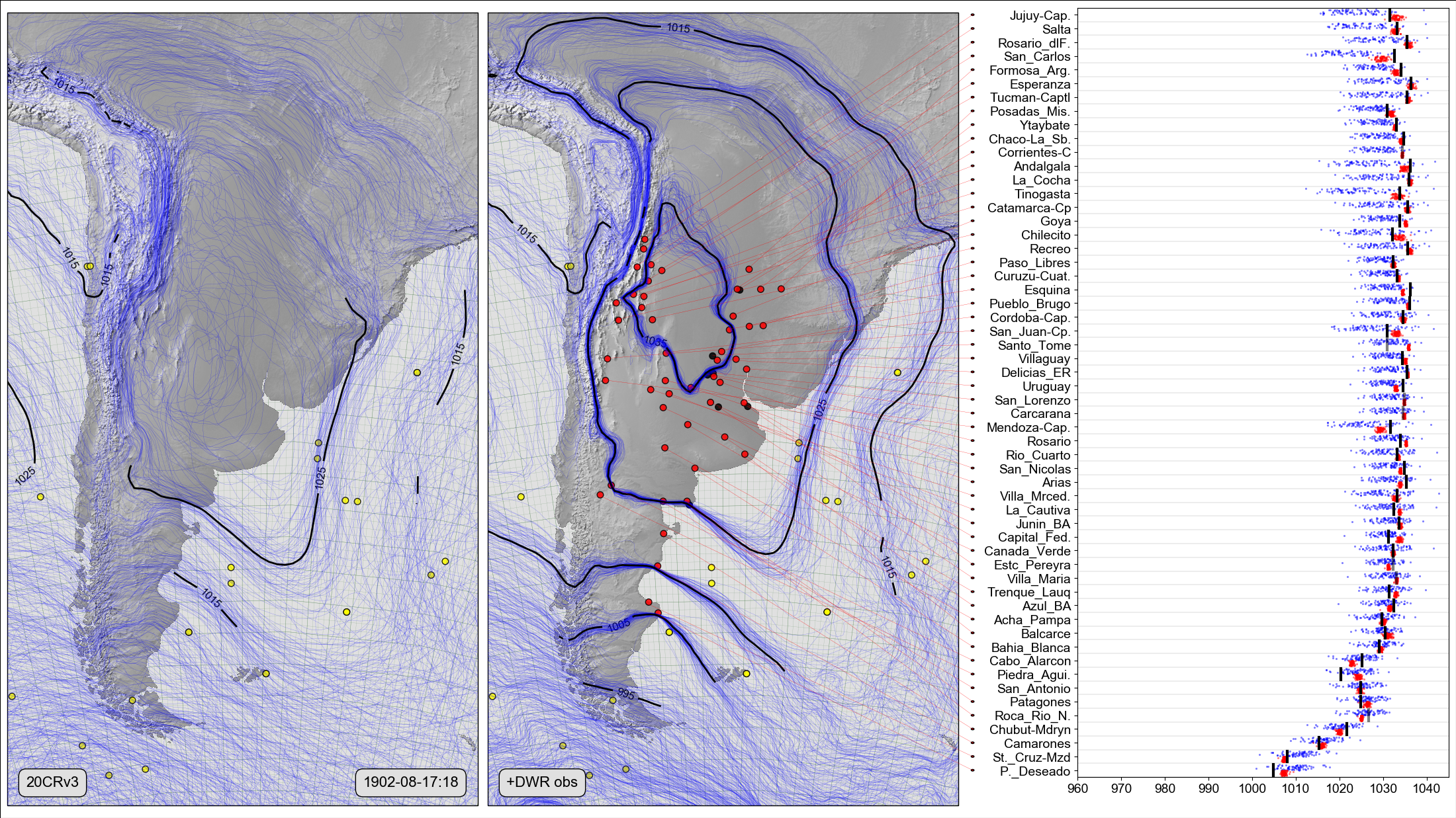
On the left, a Spaghetti-contour plot of 20CRv3 MSLP at 6 p.m. on August 17th 1902. Centre and right, Scatter-contour plot comparing the same field, after assimilating all the Argentine DWR station pressure observations within 1 hour of that date. The centre panel shows the 20CRv3 ensemble after assimilating all the station observations (red dots). The right panel compares the two ensembles with the new observations: Black lines show the observed pressures, blue dots the original 20CRv3 ensemble at the station locations, and red dots the 20CR ensemble after assimilating all the observations except the observation at that location.
Code to make the figure
Collect the reanalysis data (prmsl ensemble and observations from 20CRv3 for February 1903):
#!/usr/bin/env python

import IRData.twcr as twcr
import datetime

dte=datetime.datetime(1902,8,1)
for version in (['4.5.1']):
    twcr.fetch('prmsl',dte,version=version)
    twcr.fetch('air.2m',dte,version=version)
    twcr.fetch('tmp',dte,level=925,version=version)
    twcr.fetch_observations(dte,version=version)
Script to calculate a leave-one-out assimilation for one station:
#!/usr/bin/env python

# Assimilate all but one station for a given date
#   and store the resulting field.

import os
import math
import datetime
import numpy
import pandas
import pickle

import iris
import iris.analysis

import IRData.twcr as twcr

import SEF
import glob
import DIYA
import sklearn
RANDOM_SEED = 5

# Try and get round thread errors on spice
import dask
dask.config.set(scheduler='single-threaded')

obs_error=5 # Pa
model=sklearn.linear_model.Lasso(normalize=True)
skip_stations=['DWR_Roca_Rio_N.','DWR_Sierra_Grnde',
               'DWR_Villa_Maria','DWR_Santo_Tome','DWR_Corrientes-C',
               'DWR_Santa_Fa-Cp','DWR_San_Lorenzo','DWR_Carcarana',
               'DWR_Estc_Pereyra','DWR_Puerto_Mili.']

opdir="%s/images/ADWR_jacknife" % os.getenv('SCRATCH')
if not os.path.isdir(opdir):
    os.makedirs(opdir)

# Assimilate observations within this range of the field
hours_before=12
hours_after=12

# Get the datetime, and station to omit, from commandline arguments
import argparse
parser = argparse.ArgumentParser()
parser.add_argument("--year", help="Year",
                    type=int,required=True)
parser.add_argument("--month", help="Integer month",
                    type=int,required=True)
parser.add_argument("--day", help="Day of month",
                    type=int,required=True)
parser.add_argument("--hour", help="Time of day (0,3,6,9,12,18,or 21)",
                    type=int,required=True)
parser.add_argument("--omit", help="Name of station to be left out",
                    default=None,
                    type=str,required=False)
args = parser.parse_args()

dte=datetime.datetime(args.year,args.month,args.day,
                      int(args.hour),int(args.hour%1*60))

# 20CRv3 data
prmsl=twcr.load('prmsl',dte,version='4.5.1')

# Get the DWR observations close to the selected time
ob_start=dte-datetime.timedelta(hours=hours_before)
ob_end=dte+datetime.timedelta(hours=hours_after)
adf=glob.glob('../../../../../station-data/ToDo/sef/Argentinian_DWR/1902/DWR_*_MSLP.tsv')
obs={'name': [], 'latitude': [], 'longitude': [], 'value' : [], 'dtm' : []}
for file in adf:
   stobs=SEF.read_file(file)
   df=stobs['Data']
   # Add the datetime
   df=df.assign(Hour=(df['HHMM']/100).astype(int))
   df=df.assign(Minute=(df['HHMM']%100).astype(int))
   df=df.assign(dtm=pandas.to_datetime(df[['Year','Month','Day','Hour','Minute']]))
   # Select the subset close to the selected time
   mslp=df[(df.dtm>=ob_start) & (df.dtm<ob_end)]
   if mslp.empty: continue
   if mslp['Value'].values[0]==mslp['Value'].values[0]:
       obs['name'].append(stobs['ID'])
       obs['latitude'].append(stobs['Lat'])
       obs['longitude'].append(stobs['Lon'])
       obs['value'].append(mslp['Value'].values[0])
       obs['dtm'].append(mslp['dtm'].values[0])
obs=pandas.DataFrame(obs)

# Throw out the suspected duds
obs=obs[~obs['name'].isin(skip_stations)]
# Throw out the specified station
if args.omit is not None:
   obs=obs[~obs['name'].isin([args.omit])]

# Convert to normalised value same as reanalysis
obs.value=obs.value*100

# Update mslp by assimilating all obs.
prmsl2=DIYA.constrain_cube(prmsl,
                           lambda dte: twcr.load('prmsl',dte,version='4.5.1'),
                           obs=obs,
                           obs_error=obs_error,
                           random_state=RANDOM_SEED,
                           model=model,
                           lat_range=(-80,10),
                           lon_range=(250,350))

dumpfile="%s/%04d%02d%02d%02d.pkl" % (opdir,args.year,args.month,
                                      args.day,args.hour)
if args.omit is not None:
    dumpfile="%s/%04d%02d%02d%02d_%s.pkl" % (opdir,args.year,args.month,
                                             args.day,args.hour,args.omit)

pickle.dump( prmsl2, open( dumpfile, "wb" ) )
Calculate the leave-one-out assimilations for all the stations. (This script produces a list of calculations which can be done in parallel):
#!/usr/bin/env python

# Do all the jacknife assimilations for a range of times
# Just generates the commands to run - run with gnu parallel or similar.

import os
import sys
import time
import subprocess
import datetime
import glob
import SEF
import pandas
import numpy
from collections import OrderedDict

# Assimilate observations within this range of the field
hours_before=12
hours_after=12

# Where to put the output files
opdir="%s/images/ADWR_jacknife_png" % os.getenv('SCRATCH')
if not os.path.isdir(opdir):
    os.makedirs(opdir)

# Function to check if the job is already done for this time+omitted station
def is_done(dte,omit):
    opfile="%s/%04d%02d%02d%02d.png" % (opdir,dte.year,dte.month,
                                        dte.day,dte.hour)
    if omit is not None:
        opfile="%s/%04d%02d%02d%02d_%s.pkl" % (opdir,dte.year,dte.month,
                                               dte.day,dte.hour,omit)
    if os.path.isfile(opfile):
        return True
    return False

f=open("run.txt","w+")

start_day=datetime.datetime(1902, 8, 19, 18)
end_day  =datetime.datetime(1902, 8, 19, 18)

dte=start_day
while dte<=end_day:

    # What stations do we need to do at this point in time?
    # Load all the Argentine DWR pressures at this time
    adf=glob.glob('../../../../../station-data/ToDo/sef/Argentinian_DWR/1902/DWR_*_MSLP.tsv')
    obs={'Name': [], 'Latitude': [], 'Longitude': [], 'mslp' : []}
    for file in adf:
       stobs=SEF.read_file(file)
       df=stobs['Data']
       hhmm=int("%2d%02d" % (dte.hour,17))
       mslp=df.loc[(df['Year'] == dte.year) &
                   (df['Month'] == dte.month) &
                   (df['Day'] == dte.day) &
                   (df['HHMM'] == hhmm) ]
       if mslp.empty: continue
       if mslp['Value'].values[0]==mslp['Value'].values[0]:
           obs['Name'].append(stobs['ID'])
           obs['Latitude'].append(stobs['Lat'])
           obs['Longitude'].append(stobs['Lon'])
           obs['mslp'].append(mslp['Value'].values[0])
    obs=pandas.DataFrame(obs)
    stations=obs.Name.values.tolist()
    stations=list(OrderedDict.fromkeys(obs.Name.values))
    stations.append(None) # Also do case with all stations

    for station in stations:

        if is_done(dte,station): continue

        cmd="./leave-one-out.py --year=%d --month=%d --day=%d --hour=%d" % (
                  dte.year,dte.month,dte.day,dte.hour)
        if station is not None:
            cmd="%s --omit=%s" % (cmd,station)
        cmd="%s\n" % cmd
        f.write(cmd)
    dte=dte+datetime.timedelta(hours=24)
f.close()
Plot the figure:
#!/usr/bin/env python

# Asimilation plot for the Argentine DWRs in 1902

import os
import math
import datetime
import numpy
import pandas
import pickle
from collections import OrderedDict

import iris
import iris.analysis

import matplotlib
from matplotlib.backends.backend_agg import \
             FigureCanvasAgg as FigureCanvas
from matplotlib.figure import Figure
from matplotlib.patches import Circle

import cartopy
import cartopy.crs as ccrs

import Meteorographica as mg
import IRData.twcr as twcr

import SEF
import glob

# Try and get round thread errors on spice
import dask
dask.config.set(scheduler='single-threaded')

skip_stations=['DWR_Roca_Rio_N.','DWR_Sierra_Grnde',
               'DWR_Villa_Maria','DWR_Santo_Tome','DWR_Corrientes-C',
               'DWR_Santa_Fa-Cp','DWR_San_Lorenzo','DWR_Carcarana',
               'DWR_Estc_Pereyra','DWR_Puerto_Mili.']

# Where are the precalculated fields?
ipdir="%s/images/ADWR_jacknife" % os.getenv('SCRATCH')

# Date to show
year=1902
month=8
day=17
hour=18
minute=0 # obs are at 18:17 UTC, but show the field at 18:00
dte=datetime.datetime(year,month,day,hour,minute)

# Load all the Argentine DWR pressures at this time
adf=glob.glob('../../../../../station-data/ToDo/sef/Argentinian_DWR/1902/DWR_*_MSLP.tsv')
obs={'Name': [], 'Latitude': [], 'Longitude': [], 'mslp' : []}
for file in adf:
   stobs=SEF.read_file(file)
   df=stobs['Data']
   hhmm=int("%2d%02d" % (dte.hour,17))
   mslp=df.loc[(df['Year'] == dte.year) &
               (df['Month'] == dte.month) &
               (df['Day'] == dte.day) &
               (df['HHMM'] == hhmm) ]
   if mslp.empty: continue
   if mslp['Value'].values[0]==mslp['Value'].values[0]:
       obs['Name'].append(stobs['ID'])
       obs['Latitude'].append(stobs['Lat'])
       obs['Longitude'].append(stobs['Lon'])
       obs['mslp'].append(mslp['Value'].values[0])
obs=pandas.DataFrame(obs)

# Landscape page
aspect=16/9.0
fig=Figure(figsize=(22,22/aspect),  # Width, Height (inches)
           dpi=100,
           facecolor=(0.88,0.88,0.88,1),
           edgecolor=None,
           linewidth=0.0,
           frameon=False,
           subplotpars=None,
           tight_layout=None)
canvas=FigureCanvas(fig)
font = {'family' : 'sans-serif',
        'sans-serif' : 'Arial',
        'weight' : 'normal',
        'size'   : 14}
matplotlib.rc('font', **font)

# South America centred projection
projection=ccrs.RotatedPole(pole_longitude=120, pole_latitude=125)
scale=25
extent=[scale*-1*aspect/3.0,scale*aspect/3.0,scale*-1,scale]

# On the left - spaghetti-contour plot of original 20CRv3
ax_left=fig.add_axes([0.005,0.01,0.323,0.98],projection=projection)
ax_left.set_axis_off()
ax_left.set_extent(extent, crs=projection)
ax_left.background_patch.set_facecolor((0.88,0.88,0.88,1))
mg.background.add_grid(ax_left)
land_img_left=ax_left.background_img(name='GreyT', resolution='low')

# 20CRv3 data
prmsl=twcr.load('prmsl',dte,version='4.5.1')

# 20CRv3 data
prmsl=twcr.load('prmsl',dte,version='4.5.1')
obs_t=twcr.load_observations_fortime(dte,version='4.5.1')

# Plot the observations
mg.observations.plot(ax_left,obs_t,radius=0.2)

# PRMSL spaghetti plot
mg.pressure.plot(ax_left,prmsl,scale=0.01,type='spaghetti',
                   resolution=0.25,
                   levels=numpy.arange(875,1050,10),
                   colors='blue',
                   label=False,
                   linewidths=0.1)

# Add the ensemble mean - with labels
prmsl_m=prmsl.collapsed('member', iris.analysis.MEAN)
prmsl_s=prmsl.collapsed('member', iris.analysis.STD_DEV)
prmsl_m.data[numpy.where(prmsl_s.data>300)]=numpy.nan
mg.pressure.plot(ax_left,prmsl_m,scale=0.01,
                   resolution=0.25,
                   levels=numpy.arange(875,1050,10),
                   colors='black',
                   label=True,
                   linewidths=2)

mg.utils.plot_label(ax_left,
              '20CRv3',
              fontsize=16,
              facecolor=fig.get_facecolor(),
              x_fraction=0.04,
              horizontalalignment='left')

mg.utils.plot_label(ax_left,
              '%04d-%02d-%02d:%02d' % (year,month,day,hour),
              fontsize=16,
              facecolor=fig.get_facecolor(),
              x_fraction=0.96,
              horizontalalignment='right')

# In the centre - spaghetti-contour plot of 20CRv3 with DWR assimilated
ax_centre=fig.add_axes([0.335,0.01,0.323,0.98],projection=projection)
ax_centre.set_axis_off()
ax_centre.set_extent(extent, crs=projection)
ax_centre.background_patch.set_facecolor((0.88,0.88,0.88,1))
mg.background.add_grid(ax_centre)
land_img_centre=ax_centre.background_img(name='GreyT', resolution='low')

# Get the DWR observations for that afternoon
#obs.mslp=obs.mslp*100
obs_s=obs

# Load the all-stations-assimilated mslp
prmsl2=pickle.load( open( "%s/%04d%02d%02d%02d.pkl" %
                          (ipdir,dte.year,dte.month,
                                    dte.day,dte.hour), "rb" ) )

mg.observations.plot(ax_centre,obs_t,radius=0.2)
obs_s=obs[obs['Name'].isin(skip_stations)]
mg.observations.plot(ax_centre,obs_s,
                     radius=0.2,facecolor='black',
                     lat_label='Latitude',
                     lon_label='Longitude')
obs_s=obs[~obs['Name'].isin(skip_stations)]
mg.observations.plot(ax_centre,obs_s,
                     radius=0.2,facecolor='red',
                     lat_label='Latitude',
                     lon_label='Longitude')

# PRMSL spaghetti plot
mg.pressure.plot(ax_centre,prmsl2,scale=0.01,type='spaghetti',
                   resolution=0.25,
                   levels=numpy.arange(875,1050,10),
                   colors='blue',
                   label=False,
                   linewidths=0.1)

# Add the ensemble mean - with labels
prmsl_m=prmsl2.collapsed('member', iris.analysis.MEAN)
prmsl_s=prmsl2.collapsed('member', iris.analysis.STD_DEV)
prmsl_m.data[numpy.where(prmsl_s.data>300)]=numpy.nan
mg.pressure.plot(ax_centre,prmsl_m,scale=0.01,
                   resolution=0.25,
                   levels=numpy.arange(875,1050,10),
                   colors='black',
                   label=True,
                   linewidths=2)

mg.utils.plot_label(ax_centre,
              '+DWR obs',
              fontsize=16,
              facecolor=fig.get_facecolor(),
              x_fraction=0.04,
              horizontalalignment='left')


# Validation scatterplot on the right
obs=obs.sort_values(by='Latitude',ascending=False)
stations=list(OrderedDict.fromkeys(obs.Name.values))
# Need obs from a wider time-range to interpolate observed pressures
interpolate_obs=obs
ax_right=fig.add_axes([0.74,0.05,0.255,0.94])
# x-axis
xrange=[960,1045]
ax_right.set_xlim(xrange)
ax_right.set_xlabel('')

# y-axis
ax_right.set_ylim([1,len(stations)+1])
y_locations=[x+0.5 for x in range(1,len(stations)+1)]
ax_right.yaxis.set_major_locator(
              matplotlib.ticker.FixedLocator(y_locations))
ax_right.yaxis.set_major_formatter(
              matplotlib.ticker.FixedFormatter(
                  [s[4:] for s in stations]))

# Custom grid spacing
for y in range(0,len(stations)):
    ax_right.add_line(matplotlib.lines.Line2D(
            xdata=xrange,
            ydata=(y+1,y+1),
            linestyle='solid',
            linewidth=0.2,
            color=(0.5,0.5,0.5,1),
            zorder=0))

latlon={}

# Plot the station pressures
for y in range(0,len(stations)):
    station=stations[y]
    try:
        mslp=obs[obs.Name==station].mslp.values[0]
    except Exception: continue
    if mslp is None: continue
    if station in skip_stations:
        ax_right.add_line(matplotlib.lines.Line2D(
                xdata=(mslp,mslp), ydata=(y+1.1,y+1.9),
                linestyle='solid',
                linewidth=3,
                color=(0,0,0,0.5),
                zorder=1))
    else:
        ax_right.add_line(matplotlib.lines.Line2D(
                xdata=(mslp,mslp), ydata=(y+1.1,y+1.9),
                linestyle='solid',
                linewidth=3,
                color=(0,0,0,1),
                zorder=1))

# for each station, plot the reanalysis ensemble at that station
interpolator = iris.analysis.Linear().interpolator(prmsl,
                                   ['latitude', 'longitude'])
for y in range(len(stations)):
    station=stations[y]
    ensemble=interpolator([obs[obs.Name==station].Latitude.values[0],
                           obs[obs.Name==station].Longitude.values[0]])

    ax_right.scatter(ensemble.data/100.0,
                numpy.linspace(y+1.5,y+1.9,
                              num=len(ensemble.data)),
                20,
                'blue', # Color
                marker='.',
                edgecolors='face',
                linewidths=0.0,
                alpha=0.5,
                zorder=0.5)

# For each station, plot ensemble assimilating all but that station.
for y in range(len(stations)):
    station=stations[y]
    prmsl2=pickle.load( open( "%s/%04d%02d%02d%02d_%s.pkl" %
                                   (ipdir,dte.year,dte.month,
                                    dte.day,dte.hour,station), "rb" ) )
    interpolator = iris.analysis.Linear().interpolator(prmsl2,
                                   ['latitude', 'longitude'])
    ensemble=interpolator([obs[obs.Name==station].Latitude.values[0],
                           obs[obs.Name==station].Longitude.values[0]])
    ax_right.scatter(ensemble.data/100.0,
                numpy.linspace(y+1.1,y+1.5,
                              num=len(ensemble.data)),
                20,
                'red', # Color
                marker='.',
                edgecolors='face',
                linewidths=0.0,
                alpha=0.5,
                zorder=0.5)

# Join each station name to its location on the map
# Need another axes, filling the whole fig
ax_full=fig.add_axes([0,0,1,1])
ax_full.patch.set_alpha(0.0)  # Transparent background

def pos_left(idx):
    station=stations[idx]
    rp=ax_centre.projection.transform_points(ccrs.PlateCarree(),
                              numpy.asarray(obs[obs.Name==station].Longitude.values[0]),
                              numpy.asarray(obs[obs.Name==station].Latitude.values[0]))
    new_lon=rp[:,0]
    new_lat=rp[:,1]

    result={}
    result['x']=0.335+0.323*(new_lon-(scale*-1)*aspect/3.0)/(scale*2*aspect/3.0)
    result['y']=0.01+0.98*(new_lat-(scale*-1))/(scale*2)
    return result

# Label location of a station in ax_full coordinates
def pos_right(idx):
    result={}
    result['x']=0.668
    result['y']=0.05+(0.94/len(stations))*(idx+0.5)
    return result

for i in range(len(stations)):
    p_left=pos_left(i)
    if p_left['x']<0.335 or p_left['x']>(0.335+0.323): continue
    if p_left['y']<0.005 or p_left['y']>(0.005+0.94): continue
    p_right=pos_right(i)
    ax_full.add_patch(Circle((p_right['x'],
                              p_right['y']),
                             radius=0.001,
                             facecolor=(1,0,0,1),
                             edgecolor=(0,0,0,1),
                             alpha=1,
                             zorder=1))
    ax_full.add_line(matplotlib.lines.Line2D(
            xdata=(p_left['x'],p_right['x']),
            ydata=(p_left['y'],p_right['y']),
            linestyle='solid',
            linewidth=0.2,
            color=(1,0,0,1.0),
            zorder=1))

# Output as png
fig.savefig('Leave_one_out_%04d%02d%02d%02d%02d.png' %
                                  (year,month,day,hour,minute))