Extending the climate stripes

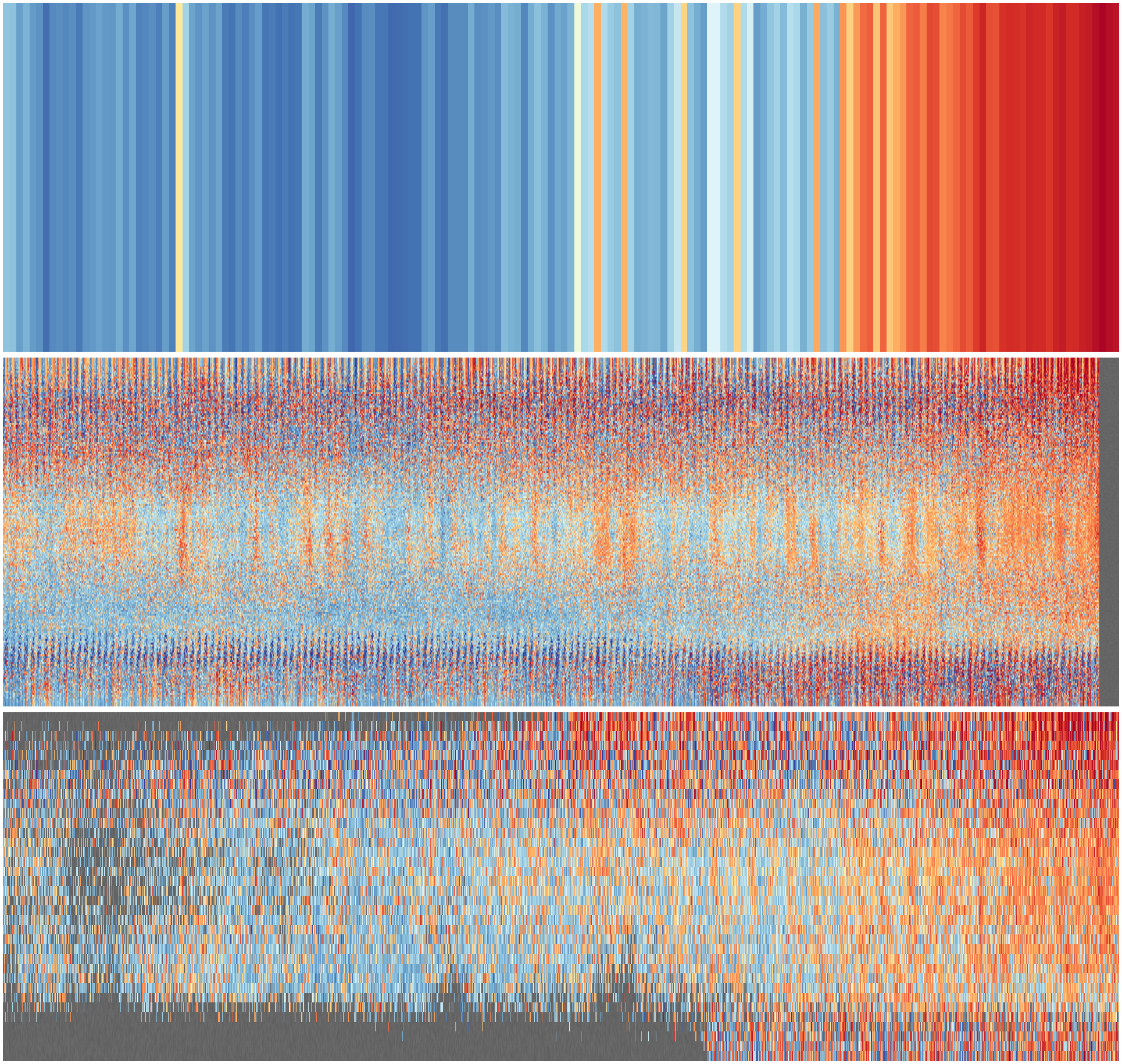
Traditional climate stripes - global-mean, annual-mean temperature anomalies (w.r.t. 1961-90) from the HadCRUT5 dataset. (Figure source).
The best response to a great idea is to steal it - to take its best parts and extend them into something new. The stripes are a great idea, but, they are deliberately simple, and so limited in what they can show - what would the professional version look like? Can we keep the clarity and power of the visualisation, while looking into the data in much more detail?
I’m making the stripes images from HadCRUT5, which provides temperature anomalies on a 5x5 degree latitude:longitude grid, every month since January 1850. To make the stripes above from this dataset requires a lot of averaging - over all latitudes and longitudes to make global means, and over the 12 months in every year to make annual means. I’d like to make a stripes plot without any averaging.
We have to make some compromises: Time:latitude:longitude is three dimensions, and we can only plot two. Time is critical, and latitude variation in temperature is generally more interesting than longitude. So let’s plot time and latitude. I don’t want to remove the longitude dimension by averaging, so instead we will sample - at each time:latitude point, choose a random longitude point to show.
Monthly temperature anomalies (w.r.t. 1961-90) from the HadCRUT5 dataset. The vertical axis is latitude (south pole at the bottom, north pole at the top), and each pixel is from a randomly selected longitude. Grey areas show regions where HadCRUT5 has no data. (Figure source).
We’ve lost some of the clarity of the original, but we can still see global warming in recent decades, and we are starting to see other things as well. However, this figure is rather noisy, and it’s missing an indication of the uncertainty of the dataset, so we need to make a couple of additional improvements:
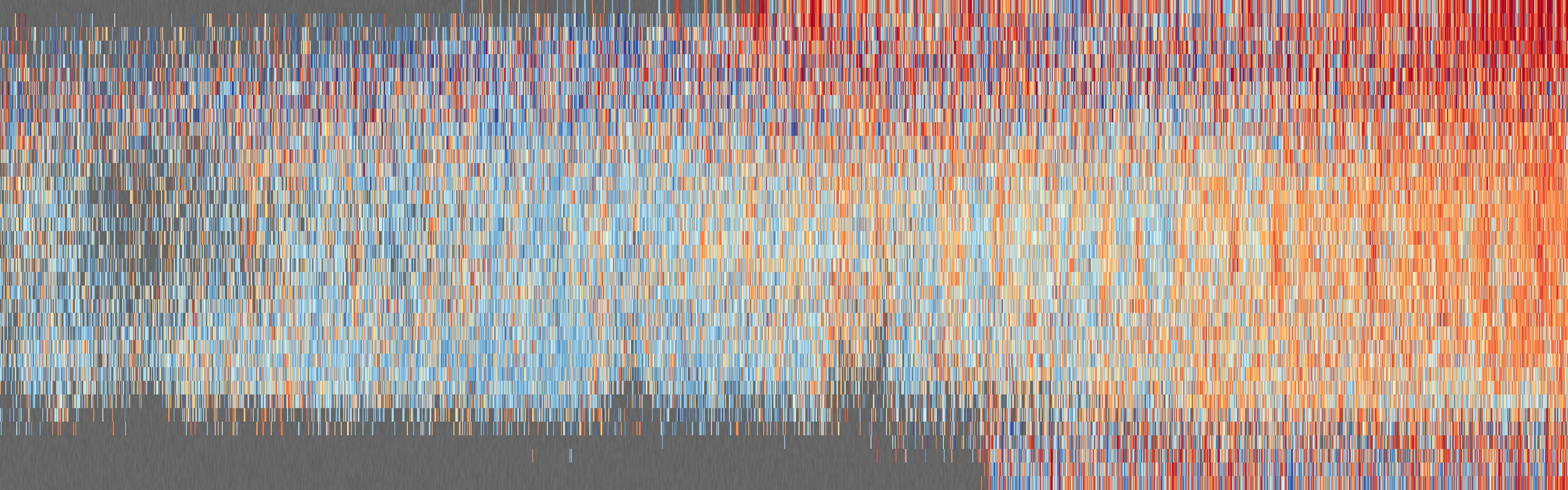
HadCRUT5 provides a metric of uncertainty by providing an ensemble of 100 posible realisations - it’s actually a four-dimensional dataset (time:latitude:longitude:ensemble). We can deal with this by sampling in the ensemble dimension as well as the longitude dimension, at each time:latitude point, choose a random longitude point, from a random ensemble member.
Also, we can reduce the noise by increasing the sampling density. If we regrid the dataset from 5 degrees in each of latitude and longitude, to 0.5 degrees, we have 10 times more latitude points to sample at. Finally, let’s add a few guidelines and labels.
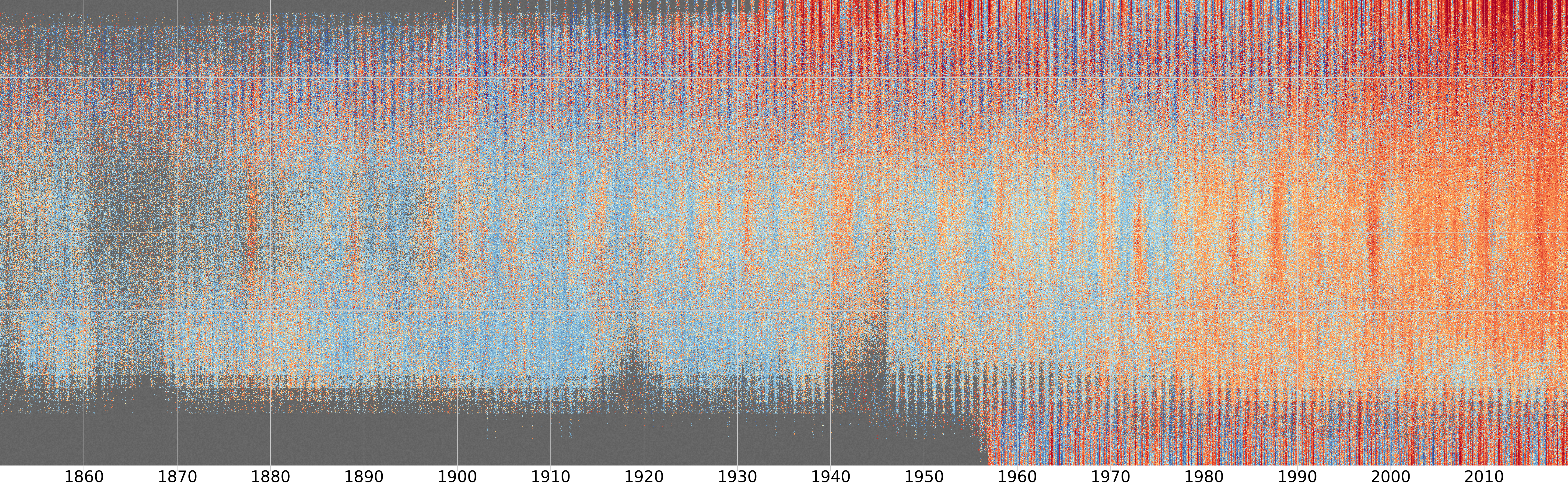
Monthly temperature anomalies (w.r.t. 1961-90) from the HadCRUT5 dataset after regridding to a 0.5 degree spatial resolution. The vertical axis is latitude (south pole at the bottom, north pole at the top), and each pixel is from a randomly selected longitude and ensemble member. Grey areas show regions where HadCRUT5 has no data. (Figure source).
In this figure red areas show time:latitude regions which were consistently warmer than normal (1961-90 average), blue shows regions where it was consistently colder, speckled areas mark regions where the warmth varied in longitude or is very uncertain (varies across the ensemble), and grey marks regions where we don’t know what it was like because we have no observations.
One instantly apparent feature of this figure are the missing observations during the "periods of reduced international cooperation". In 1861 Matthew Maury stopped collecting marine weather observations and went off to make bombs, and the resulting dent in the observations coverage lasted for more than a decade. Similar bad effects are seen over 1914-18 and 1939-46 - this "war" thing should be avoided in future. More positively, the foundation of the network of Antarctic stations in the 1950s had a marked beneficial effect in the observations coverage.
This figure shows not only the modern global warming, but variability associated with ENSO, and the marked difference in behaviour in the tropics, the southern ocean, and the high-latitude predominantly land regions. Most interestingly it shows a warming in the mid-20th century, quite different from modern global warming as it was largely restricted to the Northern high-latitudes.
This works well as an extended stripes picture, but we can further improve it:
This document and the data associated with it are crown copyright (2019) and licensed under the terms of the Open Government Licence. All code included is licensed under the terms of the GNU Lesser General Public License.