Plot image and compare data extracted by two models

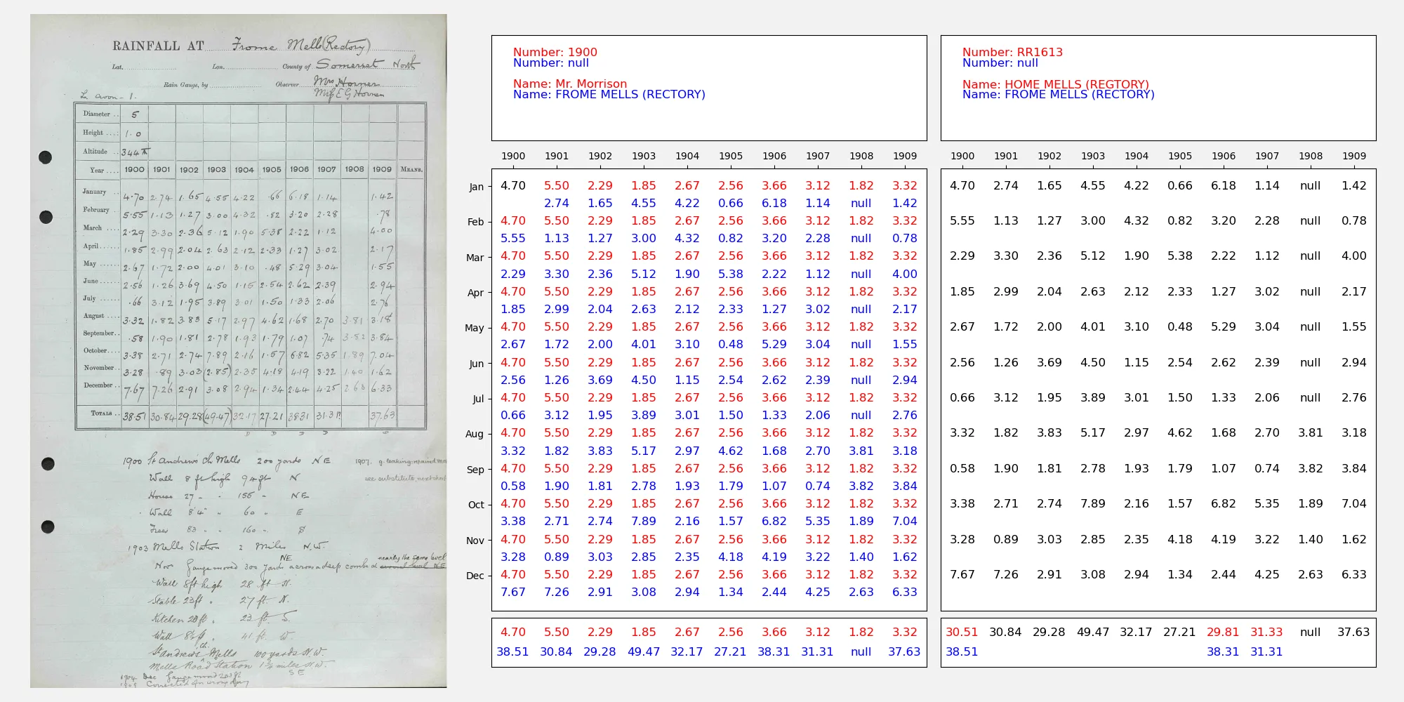
Example image and data extracted by two different models - original and fine-tuned versions of SmolVLM. Where the model extractions are right, the numbers are shown in black, where wrong, they are shown in red and the correct answer is given underneath in blue.

#!/usr/bin/env python

# Plot a 10-year monthly rainfall image and compare the data
#  two gemma versions got from it.

from rainfall_rescue.utils.pairs import get_index_list, load_pair, csv_to_json
from rainfall_rescue.utils.validate import (
    load_extracted,
    plot_image,
    plot_metadata,
    plot_monthly_table,
    plot_totals,
)
import random
import os
import re
import json
from matplotlib.backends.backend_agg import FigureCanvasAgg as FigureCanvas
from matplotlib.figure import Figure

import argparse

parser = argparse.ArgumentParser()
parser.add_argument(
    "--model_id_1",
    help="Model ID",
    type=str,
    required=False,
    default="google/gemma-3-4b-it",
)
parser.add_argument(
    "--model_id_2",
    help="Model ID",
    type=str,
    required=False,
    default="google/gemma-3-12b-it",
)
parser.add_argument(
    "--label",
    help="Image identifier",
    type=str,
    required=False,
    default=None,
)
parser.add_argument(
    "--fake",
    help="Use fake data - not real",
    action="store_true",
    required=False,
    default=False,
)
args = parser.parse_args()
if args.label is None:
    args.label = random.choice(get_index_list(fake=args.fake))

if len(args.label) < 5:
    args.fake = True

# load the image/data pair
img, csv = load_pair(args.label)
jcsv = json.loads(csv_to_json(csv))

# Load the model extracted data
extracted_1 = load_extracted(args.model_id_1, args.label)
extracted_2 = load_extracted(args.model_id_2, args.label)

# Create the figure
fig = Figure(
    figsize=(20, 10),  # Width, Height (inches)
    dpi=100,
    facecolor=(0.95, 0.95, 0.95, 1),
    edgecolor=None,
    linewidth=0.0,
    frameon=True,
    subplotpars=None,
    tight_layout=None,
)
canvas = FigureCanvas(fig)

# Image in the left
ax_original = fig.add_axes([0.01, 0.02, 0.32, 0.96])
plot_image(ax_original, img)

# First model in the middle
ax_metadata1 = fig.add_axes([0.35, 0.8, 0.31, 0.15])
plot_metadata(ax_metadata1, extracted_1, jcsv)

ax_digitised1 = fig.add_axes([0.35, 0.13, 0.31, 0.63])
plot_monthly_table(ax_digitised1, extracted_1, jcsv)

ax_totals1 = fig.add_axes([0.35, 0.05, 0.31, 0.07])
plot_totals(ax_totals1, extracted_1, jcsv)

# Second model on the right
ax_metadata2 = fig.add_axes([0.67, 0.8, 0.31, 0.15])
plot_metadata(ax_metadata2, extracted_2, jcsv)

ax_digitised2 = fig.add_axes([0.67, 0.13, 0.31, 0.63])
plot_monthly_table(ax_digitised2, extracted_2, jcsv, yticks=False)

ax_totals2 = fig.add_axes([0.67, 0.05, 0.31, 0.07])
plot_totals(ax_totals2, extracted_2, jcsv)


# Render
fig.savefig("compare.webp")