Ostia data in the Spilhaus projection
The Spilhaus projection is an ocean-centred map projection which would work nicely for displaying global marine data such as sea-surface temperatures (SST). I try, however, not to use custom projections - as far as possible I just use the equirectangular projection: It’s easy to use with the software I already have, and by suitable choice of pole location, central meridan, and scale, it’s flexible in its output.
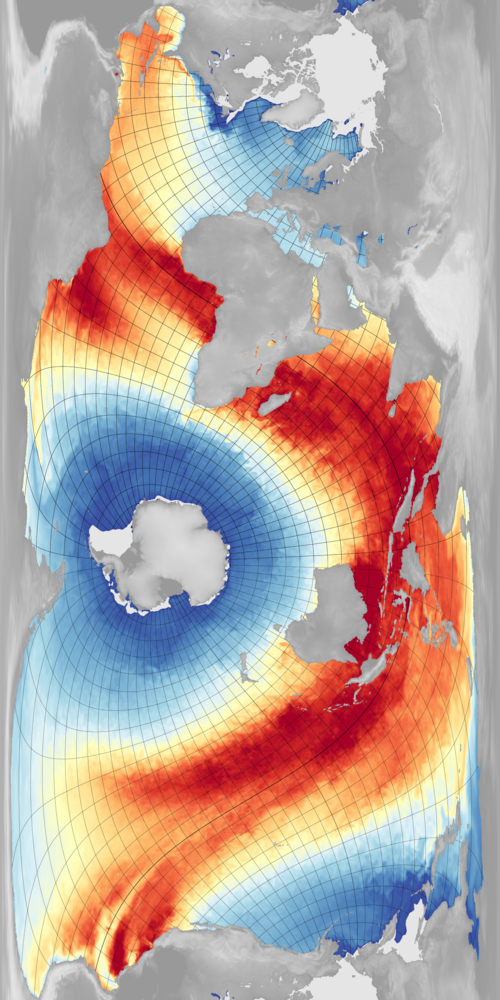
So, can we find an equirectangular approximation to the Spilhaus projection? I picked:
pole_longitude=113.0
pole_latitude=32.0
central_rotated_longitude=193.0
an extended longitude range of -202 W to 180E
Combining this with selective masking of some bits of ocean shown twice (because of the extended longitude), gave the result above. The plot is of SST from the Met Office operational model (effectively of OSTIA).
Code to make the poster
Script to download the selected data from the operational MASS archive at the Met Office:
#!/usr/bin/env python

# Retrieve surface weather variables from the global analysis
#  for one day.

import os
from tempfile import NamedTemporaryFile
import subprocess

import argparse
parser = argparse.ArgumentParser()
parser.add_argument("--year", help="Year",
                    type=int,required=True)
parser.add_argument("--month", help="Integer month",
                    type=int,required=True)
parser.add_argument("--day", help="Day of month",
                    type=int,required=True)
parser.add_argument("--opdir", help="Directory for output files",
                    default="%s/opfc/glm" % os.getenv('SCRATCH'))
args = parser.parse_args()
opdir="%s/%04d/%02d" % (args.opdir,args.year,args.month)
if not os.path.isdir(opdir):
    os.makedirs(opdir)

print("%04d-%02d-%02d" % (args.year,args.month,args.day))

# Mass directory to use
mass_dir="moose:/opfc/atm/global/prods/%04d.pp" % args.year

# Files to retrieve from
flist=[]
for hour in (0,6,12,18):
    for fcst in (0,3,6):
        flist.append("prods_op_gl-mn_%04d%02d%02d_%02d_%03d.pp" % (
                       args.year,args.month,args.day,hour,fcst))
        flist.append("prods_op_gl-mn_%04d%02d%02d_%02d_%03d.calc.pp" % (
                       args.year,args.month,args.day,hour,fcst))
        flist.append("prods_op_gl-up_%04d%02d%02d_%02d_%03d.calc.pp" % (
                       args.year,args.month,args.day,hour,fcst))

# Create the query file
qfile=NamedTemporaryFile(mode='w+',delete=False)
qfile.write("begin_global\n")
qfile.write("   pp_file = (")
for ppfl in flist:
    qfile.write("\"%s\"" % ppfl)
    if ppfl != flist[-1]:
        qfile.write(",")
    else:
        qfile.write(")\n")
qfile.write("end_global\n")
qfile.write("begin\n")
qfile.write("    stash = (16222,24,3236,31,3225,3226)\n")
qfile.write("    lbproc = 0\n")
qfile.write("end\n")
qfile.write("begin\n")
qfile.write("    stash = (5216,5206,5205,4203,4204)\n")
qfile.write("    lbproc = 128\n")
qfile.write("end\n")
qfile.close()

# Run the query
opfile="%s/%02d.pp" % (opdir,args.day)
subprocess.call("moo select -C %s %s %s" % (qfile.name,mass_dir,opfile),
                 shell=True)

os.remove(qfile.name)
Script to download the fixed land mask and orography fields:
#!/usr/bin/env python

# Download boundary conditions.
# Store it on $SCRATCH

import os
import urllib.request

# Land mask
srce=("https://s3-eu-west-1.amazonaws.com/"+
      "philip.brohan.org.big-files/fixed_fields/"+
      "land_mask/opfc_global_2019.nc")
dst="%s/fixed_fields/land_mask/opfc_global_2019.nc" % os.getenv('SCRATCH')
if not os.path.exists(dst):
    if not os.path.isdir(os.path.dirname(dst)):
        os.makedirs(os.path.dirname(dst))
    urllib.request.urlretrieve(srce, dst)
# Orography
srce=("https://s3-eu-west-1.amazonaws.com/"+
      "philip.brohan.org.big-files/fixed_fields/"+
      "orography/opfc_global_2019.nc")
dst="%s/fixed_fields/orography/opfc_global_2019.nc" % os.getenv('SCRATCH')
if not os.path.exists(dst):
    if not os.path.isdir(os.path.dirname(dst)):
        os.makedirs(os.path.dirname(dst))
    urllib.request.urlretrieve(srce, dst)
Script to plot the poster:
#!/usr/bin/env python

# Ocean-centred projection. Equirectangular, but inspired by Spilhaus.
# Meto global data.

import os
import datetime
import IRData.opfc as opfc
import Meteorographica as mg
import iris
import numpy

dte=datetime.datetime(2019,3,12,6)

import matplotlib
from matplotlib.backends.backend_agg import FigureCanvasAgg as FigureCanvas
from matplotlib.figure import Figure
from matplotlib.lines import Line2D
import cartopy
import cartopy.crs as ccrs

from pandas import qcut

# Scale down the latitudinal variation in temperature
def damp_lat(sst,factor=0.5):
    s=sst.shape
    mt=numpy.min(sst.data)
    for lat_i in range(s[0]):
        lmt=numpy.mean(sst.data[lat_i,:])
        if numpy.isfinite(lmt):
            sst.data[lat_i,:] -= (lmt-mt)*factor
    return(sst)

# Load the Meto SST
sst=opfc.load('tsurf',dte,model='global')
# And the sea-ice
icec=opfc.load('icec',dte,model='global')
# And the orography
orog=iris.load_cube("%s/fixed_fields/orography/opfc_global_2019.nc" %
                                                  os.getenv('SCRATCH'))
# And the land-sea mask
mask=iris.load_cube("%s/fixed_fields/land_mask/opfc_global_2019.nc" %
                                                  os.getenv('SCRATCH'))

# Apply the LS mask to turn tsurf into SST
sst.data[mask.data>=0.5]=numpy.nan
sst.data=numpy.ma.array(sst.data,
                        mask=mask.data>0.5)
sst=damp_lat(sst,factor=0.25)

# Define the figure (page size, background color, resolution, ...
fig=Figure(figsize=(46.8,23.4),              # Width, Height (inches)
           dpi=300,
           facecolor=(0.5,0.5,0.5,1),
           edgecolor=None,
           linewidth=0.0,
           frameon=False,                # Don't draw a frame
           subplotpars=None,
           tight_layout=None)
fig.set_frameon(False)
# Attach a canvas
canvas=FigureCanvas(fig)

# Choose a pole rotation that approximates the
# Spilhaus projection - bordered by land, ocean in the middle.
projection=ccrs.RotatedPole(pole_longitude=113.0,
                                pole_latitude=32.0,
                                central_rotated_longitude=193.0)

# To plot the fields we are going to re-grid them onto a plot cube
#  with the pole rotated to a position that approximates the
#  Spilhaus projection - bordered by land, ocean in the middle.
def plot_cube(resolution):

    extent=[-202,180,-90,90]
    pole_latitude=32.0
    pole_longitude=113.0
    npg_longitude=193.0

    cs=iris.coord_systems.RotatedGeogCS(pole_latitude,
                                        pole_longitude,
                                        npg_longitude)
    lat_values=numpy.arange(extent[2],extent[3]+resolution,resolution)
    latitude = iris.coords.DimCoord(lat_values,
                                    standard_name='latitude',
                                    units='degrees_north',
                                    coord_system=cs)
    lon_values=numpy.arange(extent[0],extent[1]+resolution,resolution)
    longitude = iris.coords.DimCoord(lon_values,
                                     standard_name='longitude',
                                     units='degrees_east',
                                     coord_system=cs)
    dummy_data = numpy.zeros((len(lat_values), len(lon_values)))
    plot_cube = iris.cube.Cube(dummy_data,
                               dim_coords_and_dims=[(latitude, 0),
                                                    (longitude, 1)])
    return plot_cube

pc=plot_cube(0.05)

# Mask out the duplicated SST data
def strip_dups(sst,resolution=0.25):
    scale=0.25/resolution
    s=sst.shape
    sst.data.mask[0:(int(150*scale)),0:(int(100*scale))]=True
    sst.data.mask[(int(150*scale)):(int(171*scale)),0:(int(75*scale))]=True
    sst.data.mask[(int(170*scale)):(int(190*scale)),0:(int(48*scale))]=True
    sst.data.mask[(int(190*scale)):(int(200*scale)),0:(int(40*scale))]=True
    sst.data.mask[(int(200*scale)):(int(210*scale)),0:(int(30*scale))]=True
    sst.data.mask[(int(210*scale)):(int(225*scale)),0:(int(15*scale))]=True
    sst.data.mask[(int(350*scale)):(int(475*scale)),0:(int(30*scale))]=True
    sst.data.mask[(int(540*scale)):,0:(int(50*scale))]=True
    for lat_in in range(0,int(300*scale)):
        for lon_in in range(s[1]-22*int(1/resolution),s[1]):
            if sst.data.mask[lat_in,lon_in-(360*int(1/resolution))]==False:
                sst.data.mask[lat_in,lon_in]=True
    return(sst)

# Define an axes to contain the plot. In this case our axes covers
#  the whole figure
ax = fig.add_axes([0,0,1,1])
ax.set_axis_off() # Don't want surrounding x and y axis

# Lat and lon range (in rotated-pole coordinates) for plot
ax.set_xlim(-202,180)
ax.set_ylim(-90,90)
ax.set_aspect('auto')

# Plot the SST
sst = sst.regrid(pc,iris.analysis.Linear())
# Strip out the duplicated data
sst=strip_dups(sst,resolution=0.05)
# Re-map to highlight small differences
s=sst.data.shape
sst.data=numpy.ma.array(qcut(sst.data.flatten(),100,labels=False,
                             duplicates='drop').reshape(s),
                        mask=sst.data.mask)
# Plot as a colour map
lats = sst.coord('latitude').points
lons = sst.coord('longitude').points
sst_img = ax.pcolorfast(lons, lats, sst.data,
                        cmap='RdYlBu_r',
                        alpha=1.0,
                        zorder=100)

# Draw lines of latitude and longitude
for offset in (-360,0):
    for lat in range(-90,95,5):
        lwd=0.1
        if lat%10==0: lwd=0.2
        if lat==0: lwd=1
        x=[]
        y=[]
        for lon in range(-180,181,1):
            rp=iris.analysis.cartography.rotate_pole(numpy.array(lon),
                                                     numpy.array(lat), 113, 32)
            nx=rp[0]+193+offset
            if nx>180: nx -= 360
            ny=rp[1]
            if(len(x)==0 or (abs(nx-x[-1])<10 and abs(ny-y[-1])<10)):
                x.append(nx)
                y.append(ny)
            else:
                ax.add_line(Line2D(x, y, linewidth=lwd, color=(0,0,0,1),
                                   zorder=150))
                x=[]
                y=[]
        if(len(x)>1):
            ax.add_line(Line2D(x, y, linewidth=lwd, color=(0,0,0,1),
                               zorder=150))

    for lon in range(-180,185,5):
        lwd=0.1
        if lon%10==0: lwd=0.2
        x=[]
        y=[]
        for lat in range(-90,90,1):
            rp=iris.analysis.cartography.rotate_pole(numpy.array(lon),
                                                     numpy.array(lat), 113, 32)
            nx=rp[0]+193+offset
            if nx>180: nx -= 360
            ny=rp[1]
            if(len(x)==0 or (abs(nx-x[-1])<10 and abs(ny-y[-1])<10)):
                x.append(nx)
                y.append(ny)
            else:
                ax.add_line(Line2D(x, y, linewidth=lwd, color=(0,0,0,1),
                                   zorder=150))
                x=[]
                y=[]
        if(len(x)>1):
            ax.add_line(Line2D(x, y, linewidth=lwd, color=(0,0,0,1),
                               zorder=150))


# Plot the sea ice
icec = icec.regrid(pc,iris.analysis.Nearest())
icec_img = ax.pcolorfast(lons, lats, icec.data,
                         cmap=matplotlib.colors.ListedColormap(
                                ((0.9,0.9,0.9,0),
                                 (0.9,0.9,0.9,1))),
                         vmin=0,
                         vmax=1,
                         alpha=1,
                         zorder=200)

# Plot the orography
o_colors=[]
for h in range(100):
    shade=0.6+h/300
    o_colors.append((shade,shade,shade,1))
orog = orog.regrid(pc,iris.analysis.Linear())
mask = mask.regrid(pc,iris.analysis.Linear())
orog.data = numpy.maximum(0.0,orog.data)
orog.data = numpy.ma.array(numpy.sqrt(orog.data),
                           mask=numpy.logical_and(mask.data<0.5,numpy.logical_not(sst.data.mask)))
orog_img = ax.pcolorfast(lons, lats, orog.data,
                         cmap=matplotlib.colors.ListedColormap(o_colors),
                         zorder=500)


# Render the figure as a pdf
fig.savefig('spilhaus_ostia_meto.pdf')