One station

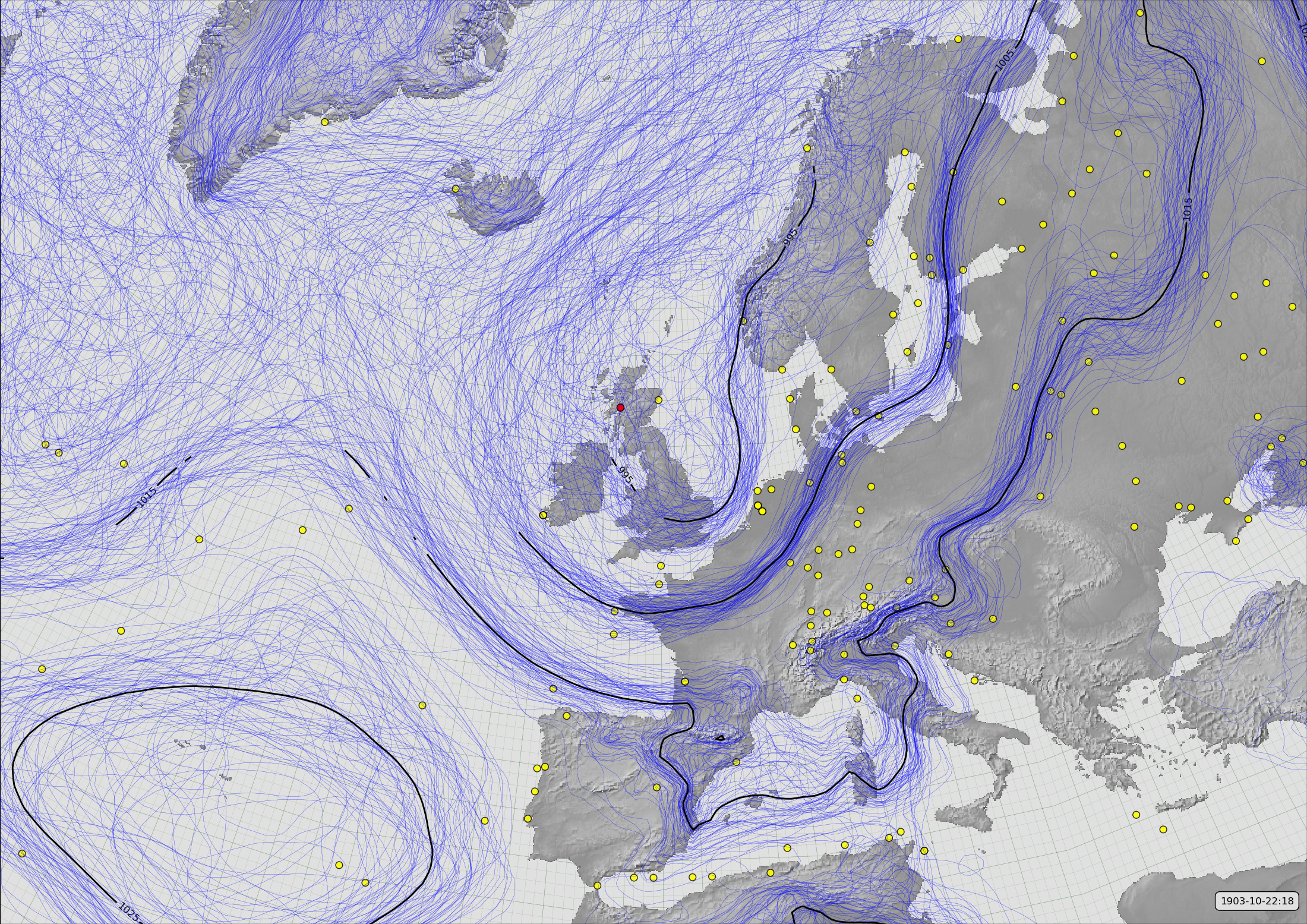
MSLP contours from 20CRv3 for October 22nd, 1903 (at 6pm), observations assimilated, yellow dots, and the location of a newly-digitised observation at Fort William (red dot).

Code to make the figure

Collect the data (prmsl ensemble and observations from 20CRv3 for October 1903):

#!/usr/bin/env python

import IRData.twcr as twcr
import datetime
dte=datetime.datetime(1903,10,22)
twcr.fetch('prmsl',dte,version='4.5.1')
twcr.fetch_observations(dte,version='4.5.1')

The Fort William location and data are in the Daily Weather Reports dataset.

Script to make the figure:

#!/usr/bin/env python

# UK region 20CRv3 spaghetti-contour prmsl map
# Show new station at Fort William

import math
import datetime
import numpy

import iris
import iris.analysis

import matplotlib
from matplotlib.backends.backend_agg import \
                FigureCanvasAgg as FigureCanvas
from matplotlib.figure import Figure

import cartopy
import cartopy.crs as ccrs

import Meteorographica as mg
import IRData.twcr as twcr

import DWR

# Date to show - low humidity at Fort William
year=1903
month=10
day=22
hour=18
dte=datetime.datetime(year,month,day,hour)

# Landscape page
fig=Figure(figsize=(22,22/math.sqrt(2)),  # Width, Height (inches)
           dpi=100,
           facecolor=(0.88,0.88,0.88,1),
           edgecolor=None,
           linewidth=0.0,
           frameon=False,
           subplotpars=None,
           tight_layout=None)
canvas=FigureCanvas(fig)

# UK-centred projection
projection=ccrs.RotatedPole(pole_longitude=177.5, pole_latitude=35.5)
scale=20
extent=[scale*-1*math.sqrt(2),scale*math.sqrt(2),scale*-1,scale]

# Single plot filling the figure
ax_20C=fig.add_axes([0,0,1,1],projection=projection)
ax_20C.set_axis_off()
ax_20C.set_extent(extent, crs=projection)

# Background, grid, and land
ax_20C.background_patch.set_facecolor((0.88,0.88,0.88,1))
mg.background.add_grid(ax_20C)
land_img_20C=ax_20C.background_img(name='GreyT', resolution='low')

# Add the observations from 20CR
obs=twcr.load_observations_fortime(dte,version='4.5.1')
mg.observations.plot(ax_20C,obs,radius=0.15)

# load the pressures
prmsl=twcr.load('prmsl',dte,version='4.5.1')

# For each ensemble member, make a contour plot
CS=mg.pressure.plot(ax_20C,prmsl,
                   resolution=0.25,
                   type='spaghetti',scale=0.01,
                   levels=numpy.arange(875,1050,10),
                   colors='blue',
                   label=False,
                   linewidths=0.2)

# Add the ensemble mean - with labels
prmsl_m=prmsl.collapsed('member', iris.analysis.MEAN)
prmsl_m.data=prmsl_m.data/100 # To hPa
prmsl_s=prmsl.collapsed('member', iris.analysis.STD_DEV)
prmsl_s.data=prmsl_s.data/100
# Mask out mean where uncertainties large
prmsl_m.data[numpy.where(prmsl_s.data>3)]=numpy.nan
CS=mg.pressure.plot(ax_20C,prmsl_m,
                   resolution=0.25,
                   levels=numpy.arange(875,1050,10),
                   colors='black',
                   label=True,
                   linewidths=2)

# Get the DWR observations within +- 2 hours
obs=DWR.load_observations('prmsl',
                          dte-datetime.timedelta(hours=2),
                          dte+datetime.timedelta(hours=2))
# Discard everthing except Fort William
obs=obs[obs.name=='FORTWILLIAM']

# Plot the Fort William station location
mg.observations.plot(ax_20C,obs,lat_label='latitude',
            lon_label='longitude',radius=0.15,facecolor='red')

mg.utils.plot_label(ax_20C,
              '%04d-%02d-%02d:%02d' % (year,month,day,hour),
              facecolor=fig.get_facecolor())
# Output as png
fig.savefig('With_FW_%04d%02d%02d%02d.png' % 
                               (year,month,day,hour))