Meteorological Data Assimilation for Data Scientists

An ensemble and an observation

Suppose we have an uncertain estimate of the weather (the mean-sea-level pressure (MSLP) field) at some point in the past, perhaps from a reanalysis, and then we get some new information, in the form of a station observation from that date and time. How can we use that new station observation to improve the MSLP estimate?

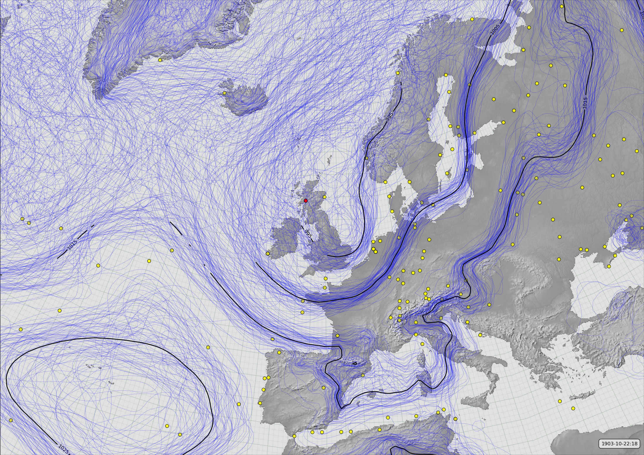
MSLP Contours for 20CR2c for October 22nd, 1903 (at 6pm).

Spaghetti-contour plot of mean-sea-level pressure, and the location of the Fort William station (red dot), where we have new observational data (Figure source).

The Ensemble Kalman Filter

We can edit the reanalysis ensemble at the location of the new observation - setting all ensemble members to the observed value, but we would like to do more than this, to use information from the observation at nearby locations as well. To decide how to modify the mslp at, say, Stornoway and London, in response to an observation at Fort William, we need to know mslp variability in those places relates to weather variability at the location of the observation. However, we can estimate this directly from the ensemble:

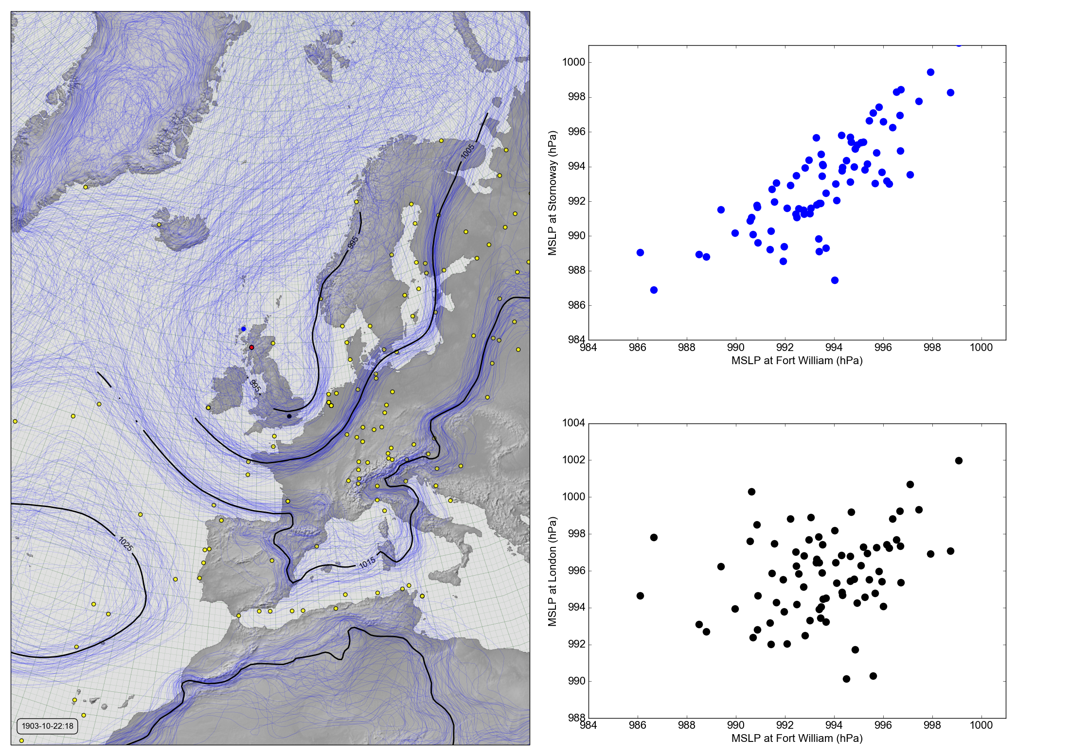
MSLP at Fort William, Stornoway, and London (October 22nd, 1903 at 6pm).

The red dot marks Fort William, the blue Stornoway, and the black London. Scatter plots show relationship between the mslp at the three locations, across the 20CRv3 ensemble, at this particular point in time. (Figure source).

In the 20CRv3 ensemble, at this point in time, the mslp at Stornoway is highly correlated with that at Fort William, so an observation at Fort William is telling us a lot about the mslp at Stornoway, and we should move the mslp estimates at Stornoway in response to the observation in much the same way as we move the estimates at Fort William. At London, on the other hand, the mslp is almost uncorrelated with that at Fort William, so an observation at Fort William is telling us little about the mslp at London, and we should leave the ensemble at London almost unchanged whatever the observation at Fort William is.

We can formalise this by fitting a model (sklearn.linear_model.LinearRegression):

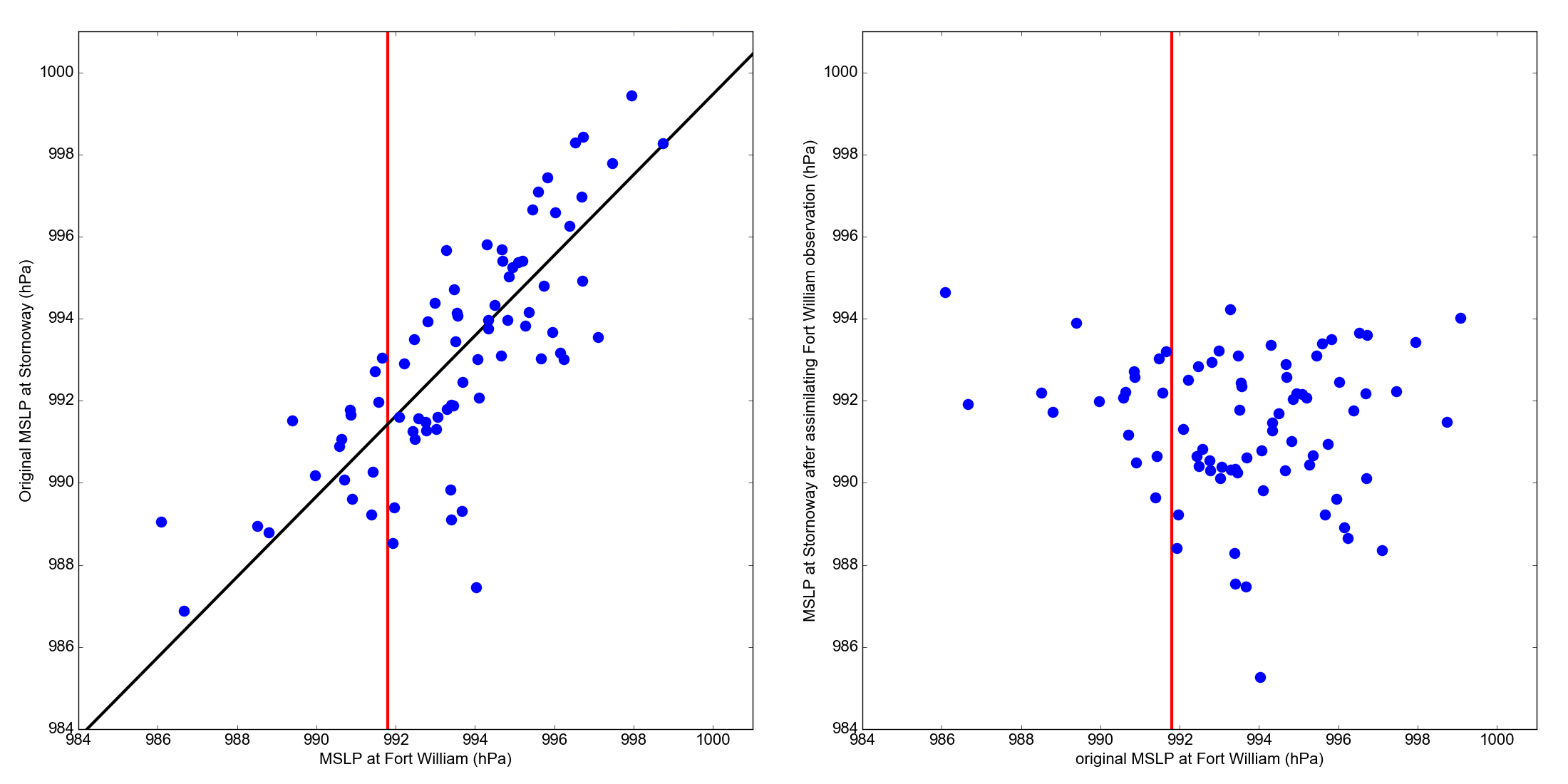
MSLP at Stornoway, before and after assimilating the Fort William observation.

Scatter plots of 20CRv3 ensemble pressures at Stornoway against ensemble pressures at Fort William, at 6pm on 22nd October 1903. The Stornoway pressures are adjusted by fitting a linear regression (left plot) and then removing the fit from each value (right plot). We can do the same for the London pressures, but in that case the adjustment will make much less difference, as the fit line has a smaller slope. (Figure source).

To fully assimilate the Fort William observation, we apply the same process illustrated above for Stornoway, to each grid-point in the reanalyis field:

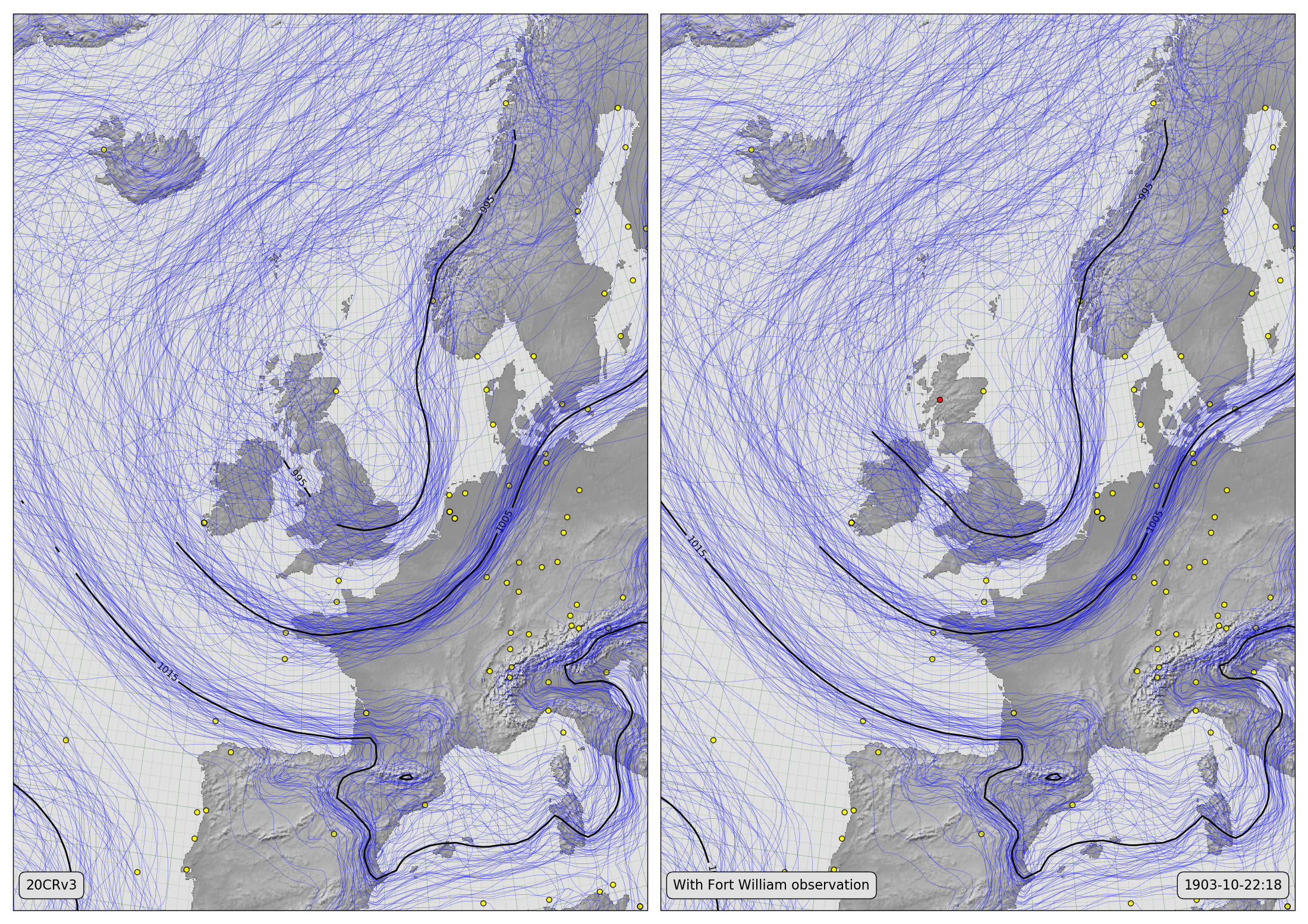
Spaghetti-contour plots showing 20CRv3 MSLP fields before (left) and after (right) assimilating Fort William observation (October 22nd, 1903 at 6pm).

The observation has pulled nearby pressures towards its value, both changing the ensemble mean and reducing the spread, while having little effect further away. (Figure source).

Validation

If it has worked well this will have improved the accuracy of the reanalysis ensemble, as well as reducing its spread. To test this, we need more observations, and fortunately the Daily Weather Reports dataset provides 22 other new obsrvations at this time, and we can compare them to the original 20CRv3 field, and to the field after assimilating the Fort William observation.

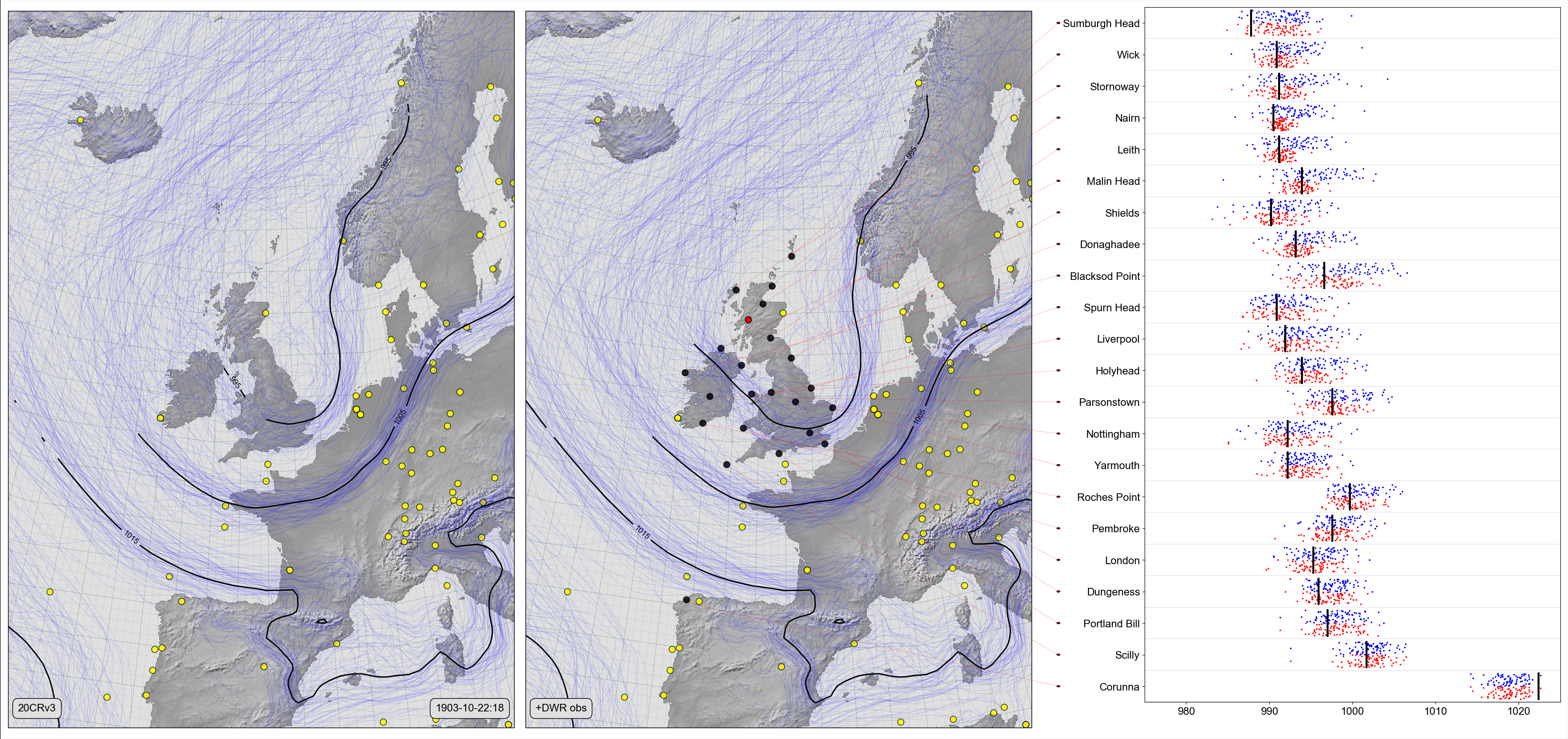
On the left, a Spaghetti-contour plot of 20CRv3 MSLP. Centre and right, Scatter-contour plot comparing the same field, after assimilating the Fort William observation, with all the other (independent) observations in the Daily Weather Reports. The centre panel shows the 20CRv3 ensemble after assimilating the Fort William observation (red dot) and the locations of all other new stations with observations at the same time (black dots). The right panel compares the two ensembles with the new observations: Black lines show the observed pressures, blue dots the original 20CRv3 ensemble at the station locations, and red dots the 20CR ensemble after assimilating the Fort William observation. (Figure source).

After assimilating the Fort William observation, the ensemble remains well calibrated to the new observations, and the ensemble spread is reduced for stations near to Fort William. So this is a success, assimilating the new observation has improved the ensemble.

Assimilating more than one observation

We can extend this same method to assimilate multiple observations, by adding an extra variable into each linear regression for each new observation.; So if we use three observations, at Fort William, Liverpool and London, we update the pressure at Stornoway by modelling the pressure at Stornoway as a multivariate linear regression on the Fort William, Liverpool and London pressures. (And validate against the remaining 20 stations):

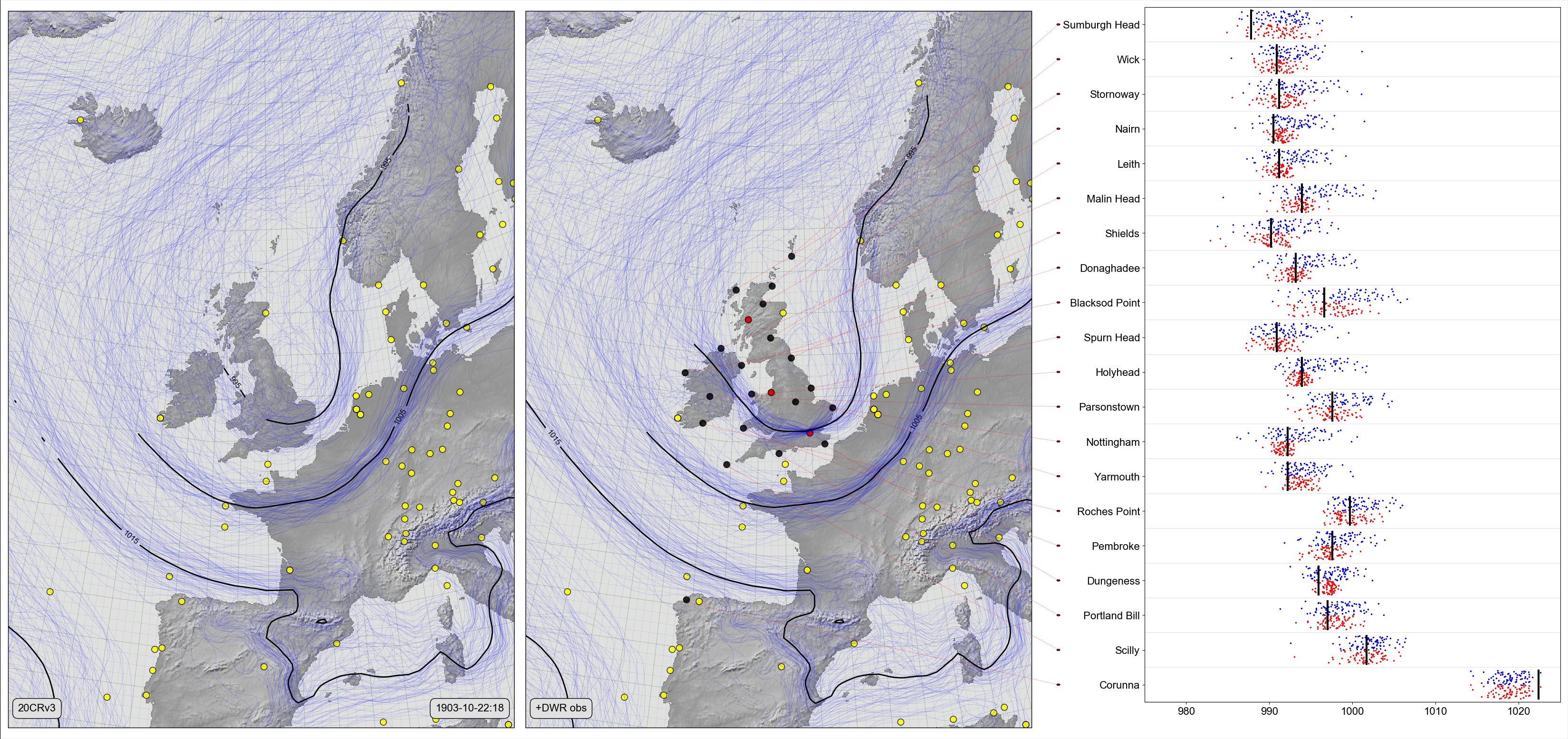
Same as the figure above, except observations from three stations (Fort William, Liverpool, and London) have been assimilated. (Figure source)

To get the best MSLP field we should assimilate all the observations, but that would leave us with nothing to validate against. A good compromise is leave-one-out validation: we do 22 assimilations, in each case assimilating all but one of the stations, and using the one left out for validation:

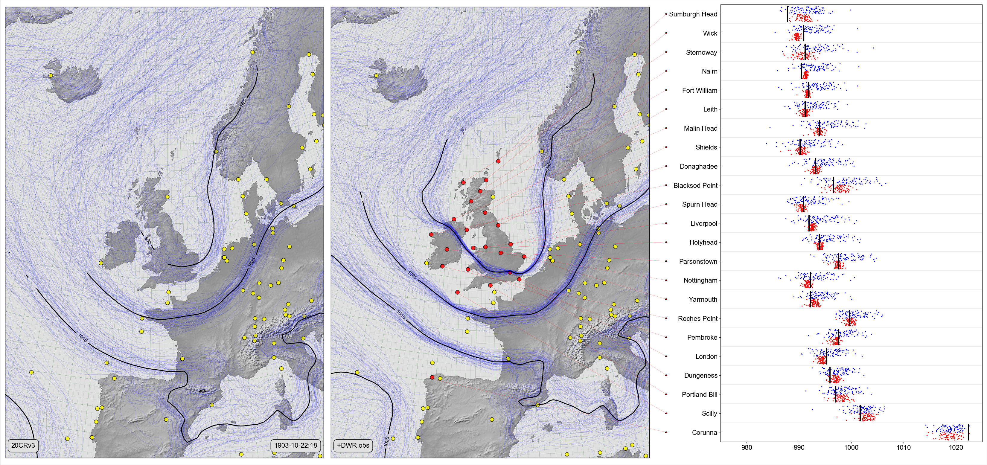
Same as the figure above, except that the centre panel shows the effect of assimilating all 22 station observations, and the right panel shows the effect, at each station, of assimilating the other 21 stations. (Figure source)