Simple weather map

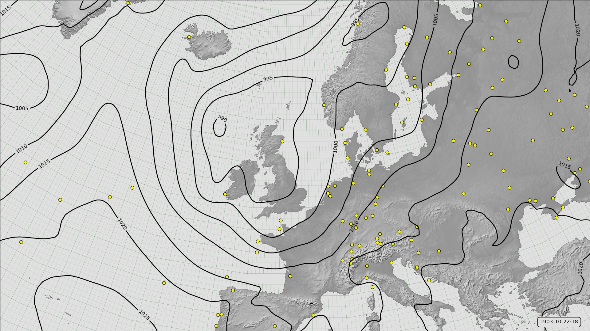
MSLP contours from the first ensemble member of 20CRv3 for October 22nd, 1903 (at 6pm), and observations assimilated.

This is a simple weather map - shows only mean-sea-level pressure (MSLP). This is a single estimate of the MSLP field.

The yellow dots show the observations assimilated into this field. |

Code to make the figure

Collect the data (prmsl ensemble and observations from 20CR2c for 1903):

#!/usr/bin/env python

import IRData.twcr as twcr
import datetime

dte=datetime.datetime(1903,10,1)
for version in (['4.5.1']):
    twcr.fetch('prmsl',dte,version=version)
    twcr.fetch_observations(dte,version=version)

Script to make the figure:

#!/usr/bin/env python

# UK region mslp single ensemble member contours for 20CRv3

import math
import datetime
import numpy
import pandas

import iris
import iris.analysis

import matplotlib
from matplotlib.backends.backend_agg import \
             FigureCanvasAgg as FigureCanvas
from matplotlib.figure import Figure

import cartopy
import cartopy.crs as ccrs

import Meteorographica as mg
import IRData.twcr as twcr

# Date to show
year=1903
month=10
day=22
hour=18
dte=datetime.datetime(year,month,day,hour)

# Landscape page
aspect=16.0/9
fig=Figure(figsize=(10.8*aspect,10.8),  # Width, Height (inches)
           dpi=100,
           facecolor=(0.88,0.88,0.88,1),
           edgecolor=None,
           linewidth=0.0,
           frameon=False,
           subplotpars=None,
           tight_layout=None)
canvas=FigureCanvas(fig)

# UK-centred projection
projection=ccrs.RotatedPole(pole_longitude=180, pole_latitude=35)
scale=15
extent=[scale*-1*aspect,scale*aspect,scale*-1,scale]

# Single plot filling figure
ax=fig.add_axes([0.0,0.0,1.0,1.0],projection=projection)
ax.set_axis_off()
ax.set_extent(extent, crs=projection)

# Background, grid and land
ax.background_patch.set_facecolor((0.88,0.88,0.88,1))
mg.background.add_grid(ax)
land_img=ax.background_img(name='GreyT', resolution='low')

# Add the observations
obs=twcr.load_observations_fortime(dte,version='4.5.1')
mg.observations.plot(ax,obs,radius=0.15)

# load the pressures
prmsl=twcr.load('prmsl',dte,version='4.5.1')

# Plot the first ensemble member - with labels
prmsl_1e=prmsl.extract(iris.Constraint(member=1))
mg.pressure.plot(ax,prmsl_1e,scale=0.01,
                   resolution=0.25,
                   levels=numpy.arange(870,1050,5),
                   colors='black',
                   label=True,
                   linewidths=2)

# label
mg.utils.plot_label(ax,
              '%04d-%02d-%02d:%02d' % (year,month,day,hour),
              facecolor=fig.get_facecolor(),
              x_fraction=0.98,
              horizontalalignment='right')

# Output as png
fig.savefig('simple_map_%04d%02d%02d%02d.png' % 
                                  (year,month,day,hour))