Simple autoencoder with fewer neurons (2 rather than 32)
The original simple autoencoder had 32 neurons in its fully-connected hidden layer. What happens if we reduce this number to 2?
#!/usr/bin/env python

# Very simple autoencoder for 20CR prmsl fields.
# Single, fully-connected layer as encoder+decoder, 32 neurons.

# This version uses only 2 neurons in the hidden layer
#   (instead of 32).

import os
import tensorflow as tf
import ML_Utilities
import pickle

# How many epochs to train for
n_epochs=100

# Create TensorFlow Dataset object from the prepared training data
(tr_data,n_steps) = ML_Utilities.dataset(purpose='training',
                                         source='20CR2c',
                                         variable='prmsl')
tr_data = tr_data.repeat(n_epochs)

# Need to reshape the data to linear, and produce a tuple
#  (source,target) for model
def to_model(ict):
   ict=tf.reshape(ict,[1,91*180])
   return(ict,ict)
tr_data = tr_data.map(to_model)

# Similar dataset from the prepared test data
(tr_test,test_steps) = ML_Utilities.dataset(purpose='test',
                                            source='20CR2c',
                                            variable='prmsl')
tr_test = tr_test.repeat(n_epochs)
tr_test = tr_test.map(to_model)

# Input placeholder - treat data as 1d
original = tf.keras.layers.Input(shape=(91*180,))
# Encoding layer 2-neuron fully-connected
encoded = tf.keras.layers.Dense(2, activation='tanh')(original)
# Output layer - same shape as input
decoded = tf.keras.layers.Dense(91*180, activation='tanh')(encoded)

# Model relating original to output
autoencoder = tf.keras.models.Model(original, decoded)
# Choose a loss metric to minimise (RMS)
#  and an optimiser to use (adadelta)
autoencoder.compile(optimizer='adadelta', loss='mean_squared_error')

# Train the autoencoder
history=autoencoder.fit(x=tr_data,
                epochs=n_epochs,
                steps_per_epoch=n_steps,
                validation_data=tr_test,
                validation_steps=test_steps,
                verbose=2) # One line per epoch

# Save the model
save_file=("%s/Machine-Learning-experiments/"+
           "simple_autoencoder_perturbations/"+
           "fewer_neurons_2/"+
           "saved_models/Epoch_%04d") % (
                 os.getenv('SCRATCH'),n_epochs)
if not os.path.isdir(os.path.dirname(save_file)):
    os.makedirs(os.path.dirname(save_file))
tf.keras.models.save_model(autoencoder,save_file)
# Save the training history
history_file=("%s/Machine-Learning-experiments/"+
              "simple_autoencoder_perturbations/"+
              "fewer_neurons_2/"+
              "/saved_models/history_to_%04d.pkl") % (
                 os.getenv('SCRATCH'),n_epochs)
pickle.dump(history.history, open(history_file, "wb"))
It should train faster, and it does; it should be noticeably less capable than the original 32-neuron version, and it is (see original):
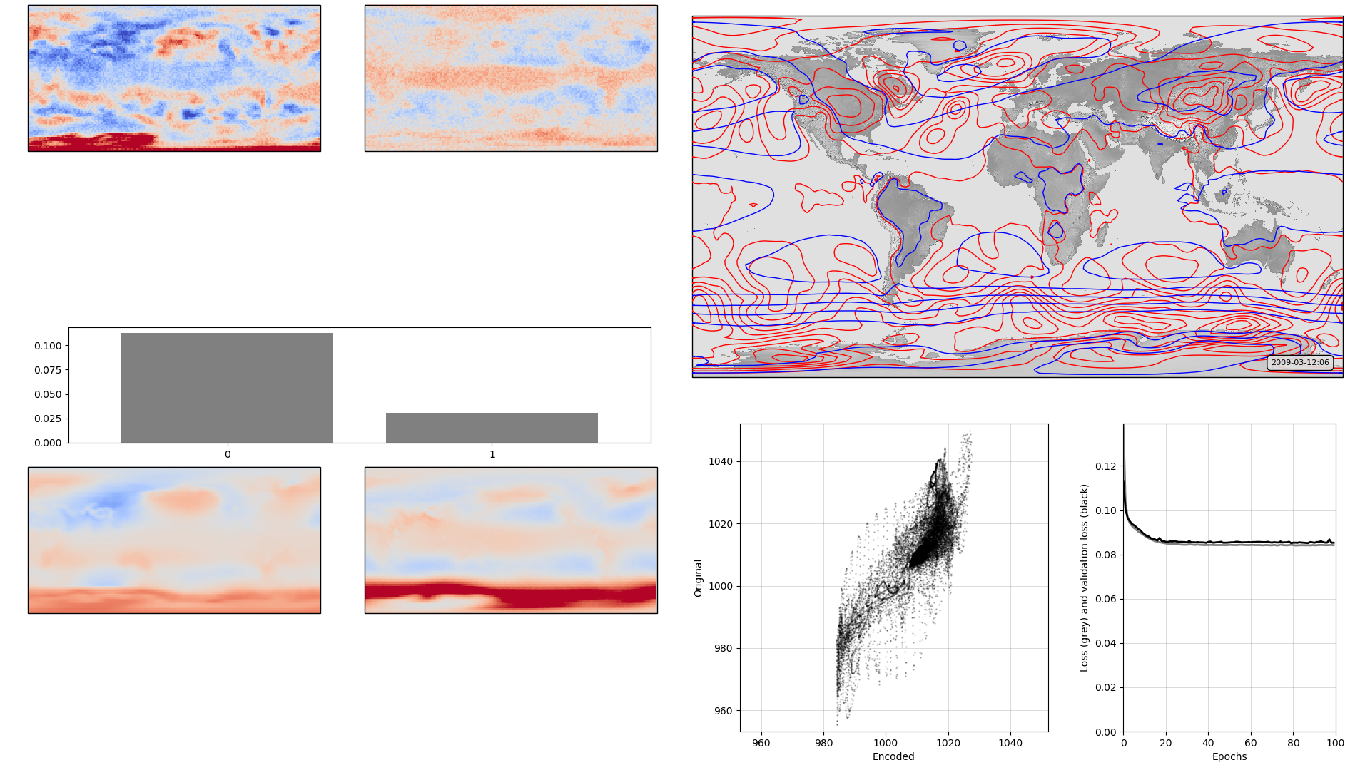
On the left, the model weights: The boxplot in the centre shows the weights associated with each neuron in the hidden layer, arranged in order, largest to smallest. Negative weights have been converted to positive (and the sign of the associated output layer weights switched accordingly). The colourmaps on top are the weights, for each hidden layer neuron, for each input field location (so a lat:lon map). They are aranged in the same order as the hidden layer weights (so if hidden-layer neuron 3 has the largest weight, the input layer weights for neuron 3 are shown at top left). The colourmaps on the bottom are the output layer weights, arranged in the same way. Top right, a sample pressure field: Original in red, after passing through the autoencoder in blue. Bottom right, training progress: Loss v. no. of training epochs.
Script to make the figure
#!/usr/bin/env python

# General model quality plot

import tensorflow as tf
tf.enable_eager_execution()
import numpy

import IRData.twcr as twcr
import iris
import datetime
import argparse
import os
import math
import pickle

import Meteorographica as mg

import matplotlib
from matplotlib.backends.backend_agg import FigureCanvasAgg as FigureCanvas
from matplotlib.figure import Figure
import cartopy
import cartopy.crs as ccrs

# Get the 20CR data
ic=twcr.load('prmsl',datetime.datetime(2009,3,12,6),
                           version='2c')
ic=ic.extract(iris.Constraint(member=1))

# Get the autoencoder
model_save_file=("%s/Machine-Learning-experiments/"+
                  "simple_autoencoder_perturbations/"+
                  "fewer_neurons_2/"+
                  "saved_models/Epoch_%04d") % (
                     os.getenv('SCRATCH'),100)
autoencoder=tf.keras.models.load_model(model_save_file)
# Get the order of the hidden weights - most to least important
order=numpy.argsort(numpy.abs(autoencoder.get_weights()[1]))[::-1]

# Normalisation - Pa to mean=0, sd=1 - and back
def normalise(x):
   x -= 101325
   x /= 3000
   return x

def unnormalise(x):
   x *= 3000
   x += 101325
   return x

fig=Figure(figsize=(19.2,10.8),  # 1920x1080, HD
           dpi=100,
           facecolor=(0.88,0.88,0.88,1),
           edgecolor=None,
           linewidth=0.0,
           frameon=False,
           subplotpars=None,
           tight_layout=None)
canvas=FigureCanvas(fig)

# Top right - map showing original and reconstructed fields
projection=ccrs.RotatedPole(pole_longitude=180.0, pole_latitude=90.0)
ax_map=fig.add_axes([0.505,0.51,0.475,0.47],projection=projection)
ax_map.set_axis_off()
extent=[-180,180,-90,90]
ax_map.set_extent(extent, crs=projection)
matplotlib.rc('image',aspect='auto')

# Run the data through the autoencoder and convert back to iris cube
pm=ic.copy()
pm.data=normalise(pm.data)
ict=tf.convert_to_tensor(pm.data, numpy.float32)
ict=tf.reshape(ict,[1,91*180]) # ????
result=autoencoder.predict_on_batch(ict)
result=tf.reshape(result,[91,180])
pm.data=unnormalise(result)

# Background, grid and land
ax_map.background_patch.set_facecolor((0.88,0.88,0.88,1))
#mg.background.add_grid(ax_map)
land_img_orig=ax_map.background_img(name='GreyT', resolution='low')

# original pressures as red contours
mg.pressure.plot(ax_map,ic,
                 scale=0.01,
                 resolution=0.25,
                 levels=numpy.arange(870,1050,7),
                 colors='red',
                 label=False,
                 linewidths=1)
# Encoded pressures as blue contours
mg.pressure.plot(ax_map,pm,
                 scale=0.01,
                 resolution=0.25,
                 levels=numpy.arange(870,1050,7),
                 colors='blue',
                 label=False,
                 linewidths=1)

mg.utils.plot_label(ax_map,
                    '%04d-%02d-%02d:%02d' % (2009,3,12,6),
                    facecolor=(0.88,0.88,0.88,0.9),
                    fontsize=8,
                    x_fraction=0.98,
                    y_fraction=0.03,
                    verticalalignment='bottom',
                    horizontalalignment='right')

# Add the model weights on the left
# Where on the plot to put each axes
def axes_geom(layer=0,channel=0,nchannels=36):
     if layer==0:
         base=[0.0,0.6,0.5,0.4]
     else:
         base=[0.0,0.0,0.5,0.4]
     ncol=math.sqrt(nchannels)
     nr=channel//ncol
     nc=channel-ncol*nr
     nr=ncol-1-nr # Top down
     geom=[base[0]+(base[2]/ncol)*0.95*nc,
           base[1]+(base[3]/ncol)*0.95*nr,
           (base[2]/ncol)*0.95,
           (base[3]/ncol)*0.95]
     geom[0] += (0.05*base[2]/(ncol+1))*(nc+1)
     geom[1] += (0.05*base[3]/(ncol+1))*(nr+1)
     return geom

# Plot a single set of weights
def plot_weights(weights,layer=0,channel=0,nchannels=36,
                 vmin=None,vmax=None):
    ax_input=fig.add_axes(axes_geom(layer=layer,
                                    channel=channel,
                                    nchannels=nchannels),
                          projection=projection)
    ax_input.set_axis_off()
    ax_input.set_extent(extent, crs=projection)
    ax_input.background_patch.set_facecolor((0.88,0.88,0.88,1))

    lats = w_in.coord('latitude').points
    lons = w_in.coord('longitude').points-180
    prate_img=ax_input.pcolorfast(lons, lats, w_in.data,
                            cmap='coolwarm',
                            vmin=vmin,
                            vmax=vmax,
                            )

# Plot the hidden layer weights
def plot_hidden(weights):
     # Single axes - var v. time
     ax=fig.add_axes([0.05,0.425,0.425,0.15])
     # Axes ranges from data
     ax.set_xlim(-0.6,len(weights)-0.4)
     ax.set_ylim(0,numpy.max(numpy.abs(weights))*1.05)
     ax.bar(x=range(len(weights)),
            height=numpy.abs(weights[order]),
            color='grey',
            tick_label=order)

plot_hidden(autoencoder.get_weights()[1])
for layer in [0,2]:
    w_l=autoencoder.get_weights()[layer]
    vmin=numpy.mean(w_l)-numpy.std(w_l)*3
    vmax=numpy.mean(w_l)+numpy.std(w_l)*3
    count=0
    for channel in order:
        w_in=ic.copy()
        if layer==0:
            w_in.data=w_l[:,channel].reshape(ic.data.shape)
        else:
            w_in.data=w_l[channel,:].reshape(ic.data.shape)
        w_in.data *= numpy.sign(autoencoder.get_weights()[1][channel])
        plot_weights(w_in,layer=layer,channel=count,nchannels=4,
                     vmin=vmin,vmax=vmax)
        count += 1

# Scatterplot of encoded v original
ax=fig.add_axes([0.54,0.05,0.225,0.4])
aspect=.225/.4*16/9
# Axes ranges from data
dmin=min(ic.data.min(),pm.data.min())
dmax=max(ic.data.max(),pm.data.max())
dmean=(dmin+dmax)/2
dmax=dmean+(dmax-dmean)*1.05
dmin=dmean-(dmean-dmin)*1.05
if aspect<1:
    ax.set_xlim(dmin/100,dmax/100)
    ax.set_ylim((dmean-(dmean-dmin)*aspect)/100,
                (dmean+(dmax-dmean)*aspect)/100)
else:
    ax.set_ylim(dmin/100,dmax/100)
    ax.set_xlim((dmean-(dmean-dmin)*aspect)/100,
                (dmean+(dmax-dmean)*aspect)/100)
ax.scatter(x=pm.data.flatten()/100,
           y=ic.data.flatten()/100,
           c='black',
           alpha=0.25,
           marker='.',
           s=2)
ax.set(ylabel='Original',
       xlabel='Encoded')
ax.grid(color='black',
        alpha=0.2,
        linestyle='-',
        linewidth=0.5)


# Plot the training history
history_save_file=("%s/Machine-Learning-experiments/"+
                   "simple_autoencoder_perturbations/"+
                   "fewer_neurons_2/"+
                   "saved_models/history_to_%04d.pkl") % (
                      os.getenv('SCRATCH'),100)
history=pickle.load( open( history_save_file, "rb" ) )
ax=fig.add_axes([0.82,0.05,0.155,0.4])
# Axes ranges from data
ax.set_xlim(0,len(history['loss']))
ax.set_ylim(0,numpy.max(numpy.concatenate((history['loss'],
                                           history['val_loss']))))
ax.set(xlabel='Epochs',
       ylabel='Loss (grey) and validation loss (black)')
ax.grid(color='black',
        alpha=0.2,
        linestyle='-',
        linewidth=0.5)
ax.plot(range(len(history['loss'])),
        history['loss'],
        color='grey',
        linestyle='-',
        linewidth=2)
ax.plot(range(len(history['val_loss'])),
        history['val_loss'],
        color='black',
        linestyle='-',
        linewidth=2)

# Render the figure as a png
fig.savefig("comparison_full.png")