Simple autoencoder for precipitation fields (instead of prmsl)
We can do prmsl, and air.2m. Let’s take on a challenge, and try precipitation.
Normalisation is difficult - I chose (rather arbitrarily), to take the square root of the rate and then multiply by 100. This gives a value between 0 and about 3.5 - with a big spike at 0.
I switched from tanh to elu activation - tanh seemed less appropriate for variables all one side of 0, but again - arbitrary choice.
I kept the RMS error metric. This is probably a poor choice - the model residuals will not be even approximately normally distributed, but it’s not obvious to me what would be better.
Otherwise - proceed as before:
#!/usr/bin/env python

# Very simple autoencoder for 20CR prmsl fields.
# Single, fully-connected layer as encoder+decoder, 32 neurons.
# Very unlikely to work well at all, but this isn't about good
#  results, it's about getting started.

# Precipitation version - the normalisation for this is a bit weird
#  as I wanted to get rid of the big spike at 0.

import os
import tensorflow as tf
#tf.enable_eager_execution()
from tensorflow.data import Dataset
from glob import glob
import numpy
import pickle

# How many times will we train on each training data point
n_epochs=100

# File names for the serialised tensors to train on
input_file_dir=(("%s/Machine-Learning-experiments/"+
                 "datasets/20CR2c/prate/training/") %
                   os.getenv('SCRATCH'))
training_files=glob("%s/*.tfd" % input_file_dir)
n_steps=len(training_files)
train_tfd = tf.constant(training_files)

# Create TensorFlow Dataset object from the file names
tr_data = Dataset.from_tensor_slices(train_tfd)

# Use all the data once each epoch
tr_data = tr_data.repeat(n_epochs)

# Present the data in random order
# ?? What does buffer_size do?
tr_data = tr_data.shuffle(buffer_size=10)

# We don't want the file names, we want their contents, so
#  add a map to convert from names to contents.
def load_tensor(file_name):
    sict=tf.read_file(file_name) # serialised
    ict=tf.parse_tensor(sict,numpy.float32)
    return ict
tr_data = tr_data.map(load_tensor)

def normalise(ic):
    ic = tf.math.sqrt(ic)
    ic *= 100
    #ic = ic+numpy.random.uniform(0,numpy.exp(-11),
    #                                           ic.shape)
    #ic = tf.math.log(ic)
    #ic += 11.5
    #ic /= 3
    #ic = tf.math.maximum(ic,-7)
    #ic = tf.math.minimum(ic,7)
    return ic

# Also need to normalise the data, reshape the data to linear, and produce a tuple
#  (source,target) for model
def to_model(ict):
   ict=normalise(tf.reshape(ict,[1,94*192]))
   return(ict,ict)
tr_data = tr_data.map(to_model)

# Make similar dataset for testing
test_file_dir=("%s/Machine-Learning-experiments/datasets/20CR2c/prate/test/" %
                   os.getenv('SCRATCH'))
test_files=glob("%s/*.tfd" % test_file_dir)
test_steps=len(test_files)
test_tfd = tf.constant(test_files)
test_data = Dataset.from_tensor_slices(test_tfd)
test_data = test_data.repeat(n_epochs)
test_data = test_data.shuffle(buffer_size=10)
test_data = test_data.map(load_tensor)
test_data = test_data.map(to_model)

# That's set up the Datasets to use - now specify an autoencoder model

# Input placeholder - treat data as 1d
original = tf.keras.layers.Input(shape=(94*192,))
# Encoding layer 32-neuron fully-connected
encoded = tf.keras.layers.Dense(32, activation='elu')(original)
# Output layer - same shape as input
decoded = tf.keras.layers.Dense(94*192, activation='elu')(encoded)

# Model relating original to output
autoencoder = tf.keras.models.Model(original, decoded)
# Choose a loss metric to minimise (RMS)
#  and an optimiser to use (adadelta)
autoencoder.compile(optimizer='adadelta', loss='mean_squared_error')

# Train the autoencoder
history=autoencoder.fit(x=tr_data, # Get (source,target) pairs from this Dataset
                        epochs=n_epochs,
                        steps_per_epoch=n_steps,
                        validation_data=test_data,
                        validation_steps=test_steps,
                        verbose=2) # One line per epoch

# Save the model
save_file=("%s/Machine-Learning-experiments/"+
           "simple_autoencoder_variables/prate/"+
           "saved_models/Epoch_%04d") % (
                 os.getenv('SCRATCH'),n_epochs)
if not os.path.isdir(os.path.dirname(save_file)):
    os.makedirs(os.path.dirname(save_file))
tf.keras.models.save_model(autoencoder,save_file)
# Save the training history
history_file=("%s/Machine-Learning-experiments/"+
              "simple_autoencoder_variables/prate/"+
              "saved_models/history_to_%04d.pkl") % (
                 os.getenv('SCRATCH'),n_epochs)
pickle.dump(history.history, open(history_file, "wb"))
Somewhat to my suprise, this does work to an extent (compare prmsl, air.2m). It’s only using 12 neurons(why)?, it’s overfitted (best at 10 epochs, why?), but it’s not hopeless. More cunning approaches to normalisation, and model parameters, might make a big improvement.
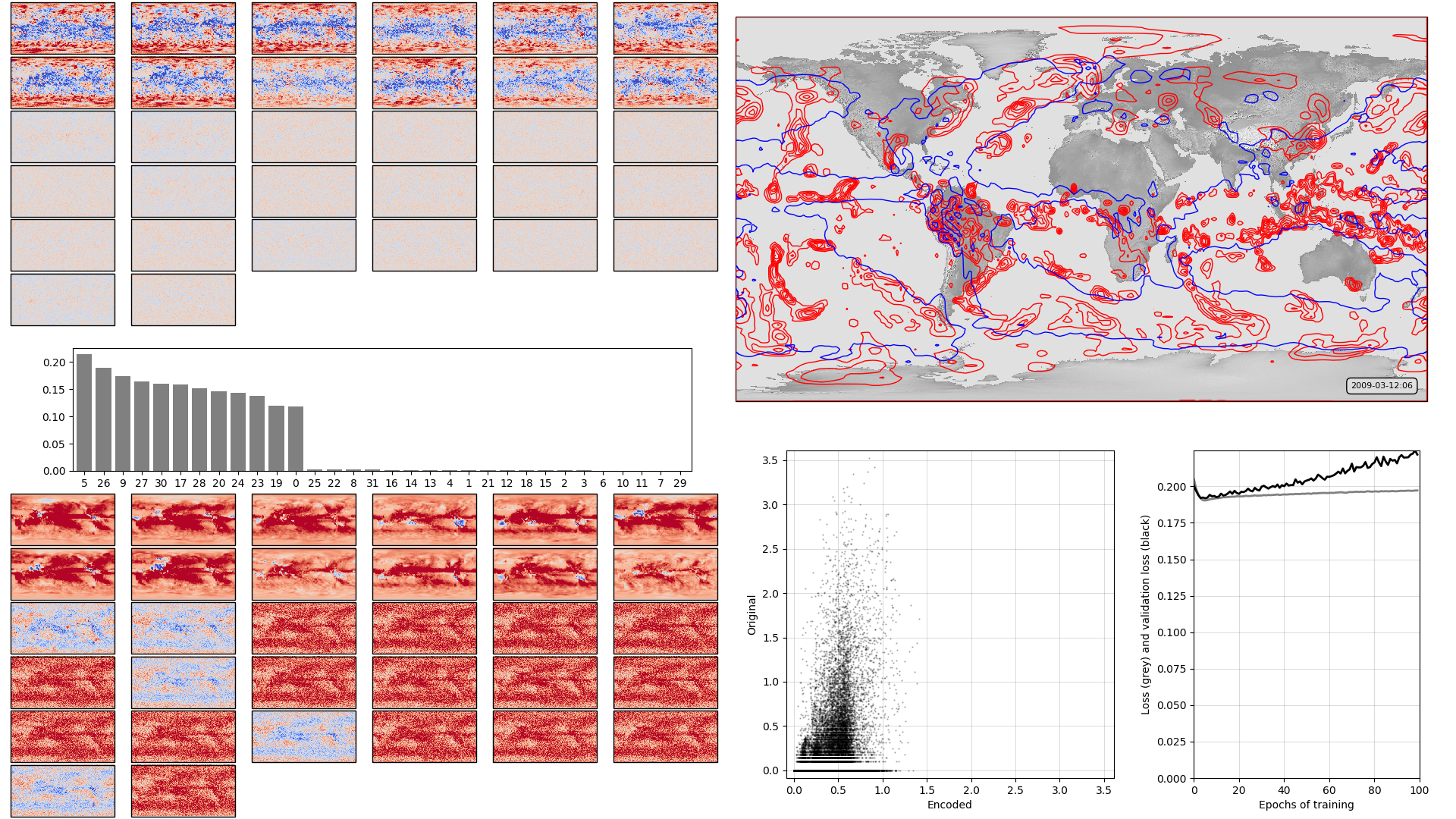
On the left, the model weights: The boxplot in the centre shows the weights associated with each neuron in the hidden layer, arranged in order, largest to smallest. Negative weights have been converted to positive (and the sign of the associated output layer weights switched accordingly). The colourmaps on top are the weights, for each hidden layer neuron, for each input field location (so a lat:lon map). They are aranged in the same order as the hidden layer weights (so if hidden-layer neuron 3 has the largest weight, the input layer weights for neuron 3 are shown at top left). The colourmaps on the bottom are the output layer weights, arranged in the same way. Top right, a sample precipitation field (note, after square-root transform): Original in red, after passing through the autoencoder in blue. Bottom right, training progress: Loss v. no. of training epochs.
Script to make the figure
#!/usr/bin/env python

# General model quality plot

import tensorflow as tf
tf.enable_eager_execution()
import numpy

import IRData.twcr as twcr
import iris
import datetime
import argparse
import os
import math
import pickle

import Meteorographica as mg

import matplotlib
from matplotlib.backends.backend_agg import FigureCanvasAgg as FigureCanvas
from matplotlib.figure import Figure
import cartopy
import cartopy.crs as ccrs

# Get the 20CR data
ic=twcr.load('prate',datetime.datetime(2009,3,12,6),
                           version='2c')
ic=ic.extract(iris.Constraint(member=1))

# Get the autoencoder
model_save_file=("%s/Machine-Learning-experiments/"+
           "simple_autoencoder_variables/prate/"+
           "saved_models/Epoch_%04d") % (
                 os.getenv('SCRATCH'),100)
autoencoder=tf.keras.models.load_model(model_save_file)
# Get the order of the hidden weights - most to least important
order=numpy.argsort(numpy.abs(autoencoder.get_weights()[1]))[::-1]

# Normalisation - Weird - because precip
def normalise(x):
    x = numpy.sqrt(x)
    x *= 100
    #x = x+numpy.random.uniform(0,numpy.exp(-11),x.shape)
    #x = numpy.log(x)
    #x += 11.5
    #x /= 3
    #x = numpy.maximum(x,-7)
    #x = numpy.minimum(x,7)
    return x

fig=Figure(figsize=(19.2,10.8),  # 1920x1080, HD
           dpi=100,
           facecolor=(0.88,0.88,0.88,1),
           edgecolor=None,
           linewidth=0.0,
           frameon=False,
           subplotpars=None,
           tight_layout=None)
canvas=FigureCanvas(fig)

# Top right - map showing original and reconstructed fields
projection=ccrs.RotatedPole(pole_longitude=180.0, pole_latitude=90.0)
ax_map=fig.add_axes([0.505,0.51,0.475,0.47],projection=projection)
ax_map.set_axis_off()
extent=[-180,180,-90,90]
ax_map.set_extent(extent, crs=projection)
matplotlib.rc('image',aspect='auto')

# Run the data through the autoencoder and convert back to iris cube
pm=ic.copy()
pm.data=normalise(pm.data)
ic.data=pm.data
ict=tf.convert_to_tensor(pm.data, numpy.float32)
ict=tf.reshape(ict,[1,94*192]) # ????
result=autoencoder.predict_on_batch(ict)
result=tf.reshape(result,[94,192])
pm.data=result

# Background, grid and land
ax_map.background_patch.set_facecolor((0.88,0.88,0.88,1))
#mg.background.add_grid(ax_map)
land_img_orig=ax_map.background_img(name='GreyT', resolution='low')

# original pressures as red contours
mg.pressure.plot(ax_map,ic,
                 scale=1,
                 resolution=0.25,
                 levels=numpy.arange(0.5,3.5,0.5),
                 colors='red',
                 label=False,
                 linewidths=1)
# Encoded pressures as blue contours
mg.pressure.plot(ax_map,pm,
                 scale=1,
                 resolution=0.25,
                 levels=numpy.arange(0.5,3.5,0.5),
                 colors='blue',
                 label=False,
                 linewidths=1)

mg.utils.plot_label(ax_map,
                    '%04d-%02d-%02d:%02d' % (2009,3,12,6),
                    facecolor=(0.88,0.88,0.88,0.9),
                    fontsize=8,
                    x_fraction=0.98,
                    y_fraction=0.03,
                    verticalalignment='bottom',
                    horizontalalignment='right')

# Add the model weights on the left
# Where on the plot to put each axes
def axes_geom(layer=0,channel=0,nchannels=36):
     if layer==0:
         base=[0.0,0.6,0.5,0.4]
     else:
         base=[0.0,0.0,0.5,0.4]
     ncol=math.sqrt(nchannels)
     nr=channel//ncol
     nc=channel-ncol*nr
     nr=ncol-1-nr # Top down
     geom=[base[0]+(base[2]/ncol)*0.95*nc,
           base[1]+(base[3]/ncol)*0.95*nr,
           (base[2]/ncol)*0.95,
           (base[3]/ncol)*0.95]
     geom[0] += (0.05*base[2]/(ncol+1))*(nc+1)
     geom[1] += (0.05*base[3]/(ncol+1))*(nr+1)
     return geom

# Plot a single set of weights
def plot_weights(weights,layer=0,channel=0,nchannels=36,
                 vmin=None,vmax=None):
    ax_input=fig.add_axes(axes_geom(layer=layer,
                                    channel=channel,
                                    nchannels=nchannels),
                          projection=projection)
    ax_input.set_axis_off()
    ax_input.set_extent(extent, crs=projection)
    ax_input.background_patch.set_facecolor((0.88,0.88,0.88,1))

    lats = w_in.coord('latitude').points
    lons = w_in.coord('longitude').points-180
    prate_img=ax_input.pcolorfast(lons, lats, w_in.data,
                            cmap='coolwarm',
                            vmin=vmin,
                            vmax=vmax,
                            )

# Plot the hidden layer weights
def plot_hidden(weights):
     # Single axes - var v. time
     ax=fig.add_axes([0.05,0.425,0.425,0.15])
     # Axes ranges from data
     ax.set_xlim(-0.6,len(weights)-0.4)
     ax.set_ylim(0,numpy.max(numpy.abs(weights))*1.05)
     ax.bar(x=range(len(weights)),
            height=numpy.abs(weights[order]),
            color='grey',
            tick_label=order)

plot_hidden(autoencoder.get_weights()[1])
for layer in [0,2]:
    w_l=autoencoder.get_weights()[layer]
    vmin=numpy.mean(w_l)-numpy.std(w_l)*3
    vmax=numpy.mean(w_l)+numpy.std(w_l)*3
    count=0
    for channel in order:
        w_in=ic.copy()
        if layer==0:
            w_in.data=w_l[:,channel].reshape(ic.data.shape)
        else:
            w_in.data=w_l[channel,:].reshape(ic.data.shape)
        w_in.data *= numpy.sign(autoencoder.get_weights()[1][channel])
        plot_weights(w_in,layer=layer,channel=count,nchannels=36,
                     vmin=vmin,vmax=vmax)
        count += 1

# Scatterplot of encoded v original
ax=fig.add_axes([0.54,0.05,0.225,0.4])
aspect=.225/.4*16/9
# Axes ranges from data
dmin=min(ic.data.min(),pm.data.min())
dmax=max(ic.data.max(),pm.data.max())
dmean=(dmin+dmax)/2
dmax=dmean+(dmax-dmean)*1.05
dmin=dmean-(dmean-dmin)*1.05
if aspect<1:
    ax.set_xlim(dmin,dmax)
    ax.set_ylim((dmean-(dmean-dmin)*aspect),
                (dmean+(dmax-dmean)*aspect))
else:
    ax.set_ylim(dmin,dmax)
    ax.set_xlim((dmean-(dmean-dmin)*aspect),
                (dmean+(dmax-dmean)*aspect))
ax.scatter(x=pm.data.flatten(),
           y=ic.data.flatten(),
           c='black',
           alpha=0.25,
           marker='.',
           s=2)
ax.set(ylabel='Original',
       xlabel='Encoded')
ax.grid(color='black',
        alpha=0.2,
        linestyle='-',
        linewidth=0.5)

# Plot the training history
history_save_file=("%s/Machine-Learning-experiments/"+
              "simple_autoencoder_variables/prate/"+
              "saved_models/history_to_%04d.pkl") % (
                  os.getenv('SCRATCH'),100)
history=pickle.load( open( history_save_file, "rb" ) )
ax=fig.add_axes([0.82,0.05,0.155,0.4])
# Axes ranges from data
ax.set_xlim(0,len(history['loss']))
ax.set_ylim(0,numpy.max(numpy.concatenate((history['loss'],
                                           history['val_loss']))))
ax.set(xlabel='Epochs of training',
       ylabel='Loss (grey) and validation loss (black)')
ax.grid(color='black',
        alpha=0.2,
        linestyle='-',
        linewidth=0.5)
ax.plot(range(len(history['loss'])),
        history['loss'],
        color='grey',
        linestyle='-',
        linewidth=2)
ax.plot(range(len(history['val_loss'])),
        history['val_loss'],
        color='black',
        linestyle='-',
        linewidth=2)

# Render the figure as a png
fig.savefig("comparison_full.png")