An all-convolutional autoencoder with better training data
The all-convolutional autoencoder is a nuisance to use, as the strided convolutions mean it’s fussy about resolution, and it’s not clear how best to deal with the data boundary conditions. The latter problem is particulary acute when using 20CR2c data, as its longitude splice is at 0/360 and so goes through the UK; so the problem is most acute where I want the results to be best.
Making a convolutional autoencoder which deals correctly with both the periodic and polar boundaries would be tricky. A much easier approach is to re-grid the training data so all the interesting points are in the middle. Regridding to a modified Cassini projection with the North pole at 90W on the equator moves the poles to the centre of the crid and puts all the boundary points on the equator. At the same time we can set the field resolution to a value which works nicely with strided convolutions.
Then the code is the same as for the all-convolutional autoencoder, except that all the complications of resixzing and padding can be removed:
#!/usr/bin/env python

# Convolutional autoencoder for 20CR prmsl fields.
# This version is all-convolutional - it uses strided convolutions
#  instead of max-pooling, and transpose convolution instead of
#  upsampling.
# This version uses scaled input fields that have a size (79x159) that
#  match the strided convolution upscaling and downscaling.
# It also works on tensors with a rotated pole - so the data boundary
#  is the equator - this limits the problems with boundary conditions.

import os
import tensorflow as tf
import ML_Utilities
import pickle
import numpy

# How many epochs to train for
n_epochs=50

# Create TensorFlow Dataset object from the prepared training data
(tr_data,n_steps) = ML_Utilities.dataset(purpose='training',
                                         source='rotated_pole/20CR2c',
                                         variable='prmsl')
tr_data = tr_data.repeat(n_epochs)

# Also produce a tuple (source,target) for model
def to_model(ict):
   ict=tf.reshape(ict,[79,159,1])
   return(ict,ict)
tr_data = tr_data.map(to_model)
tr_data = tr_data.batch(1)

# Similar dataset from the prepared test data
(tr_test,test_steps) = ML_Utilities.dataset(purpose='test',
                                            source='rotated_pole/20CR2c',
                                            variable='prmsl')
tr_test = tr_test.repeat(n_epochs)
tr_test = tr_test.map(to_model)
tr_test = tr_test.batch(1)


# Input placeholder
original = tf.keras.layers.Input(shape=(79,159,1,))
# Encoding layers
x = tf.keras.layers.Conv2D(16, (3, 3), padding='same')(original)
x = tf.keras.layers.LeakyReLU()(x)
x = tf.keras.layers.Conv2D(8, (3, 3), strides= (2,2), padding='valid')(x)
x = tf.keras.layers.LeakyReLU()(x)
x = tf.keras.layers.Conv2D(8, (3, 3), strides= (2,2), padding='valid')(x)
x = tf.keras.layers.LeakyReLU()(x)
x = tf.keras.layers.Conv2D(8, (3, 3), strides= (2,2), padding='valid')(x)
x = tf.keras.layers.LeakyReLU()(x)
encoded = x

# Decoding layers
x = tf.keras.layers.Conv2DTranspose(8, (3, 3),  strides= (2,2), padding='valid')(encoded)
x = tf.keras.layers.LeakyReLU()(x)
x = tf.keras.layers.Conv2DTranspose(8, (3, 3),  strides= (2,2), padding='valid')(x)
x = tf.keras.layers.LeakyReLU()(x)
x = tf.keras.layers.Conv2DTranspose(8, (3, 3),  strides= (2,2), padding='valid')(x)
x = tf.keras.layers.LeakyReLU()(x)
decoded = tf.keras.layers.Conv2D(1, (3, 3), padding='same')(x)

# Model relating original to output
autoencoder = tf.keras.models.Model(original,decoded)
# Choose a loss metric to minimise (RMS)
#  and an optimiser to use (adadelta)
autoencoder.compile(optimizer='adadelta', loss='mean_squared_error')

# Train the autoencoder
history=autoencoder.fit(x=tr_data,
                epochs=n_epochs,
                steps_per_epoch=n_steps,
                validation_data=tr_test,
                validation_steps=test_steps,
                verbose=2) # One line per epoch

# Save the model
save_file=("%s/Machine-Learning-experiments/"+
           "convolutional_autoencoder_perturbations/"+
           "rotated+scaled/saved_models/Epoch_%04d") % (
                 os.getenv('SCRATCH'),n_epochs)
if not os.path.isdir(os.path.dirname(save_file)):
    os.makedirs(os.path.dirname(save_file))
tf.keras.models.save_model(autoencoder,save_file)
history_file=("%s/Machine-Learning-experiments/"+
              "convolutional_autoencoder_perturbations/"+
              "rotated+scaled/saved_models/history_to_%04d.pkl") % (
                 os.getenv('SCRATCH'),n_epochs)
pickle.dump(history.history, open(history_file, "wb"))
It works pretty well, with only very minor issues near the boundaries.
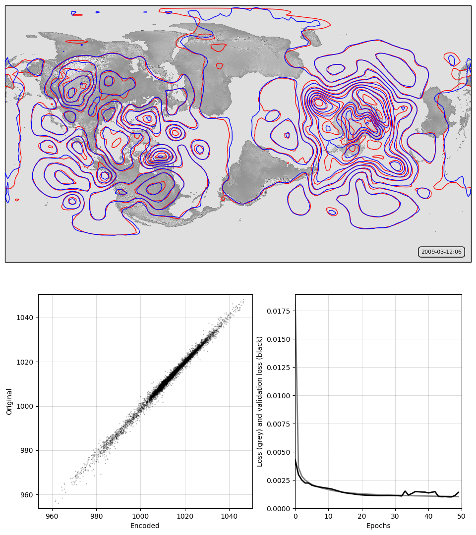
Top, a sample pressure field: Original in red, after passing through the autoencoder in blue. Bottom, a scatterplot of original v. encoded pressures for the sample field, and a graph of training progress: Loss v. no. of training epochs.
Script to make the figure
#!/usr/bin/env python

# Model training results plot

import tensorflow as tf
tf.enable_eager_execution()
import numpy

import IRData.twcr as twcr
import iris
import datetime
import argparse
import os
import math
import pickle

import Meteorographica as mg

import matplotlib
from matplotlib.backends.backend_agg import FigureCanvasAgg as FigureCanvas
from matplotlib.figure import Figure
import cartopy
import cartopy.crs as ccrs

# Function to resize and rotate pole
def rr_cube(cbe):
    # Use the Cassini projection (boundary is the equator)
    cs=iris.coord_systems.RotatedGeogCS(0.0,60.0,270.0)
    # Latitudes cover -90 to 90 with 79 values
    lat_values=numpy.arange(-90,91,180/78)
    latitude = iris.coords.DimCoord(lat_values,
                                    standard_name='latitude',
                                    units='degrees_north',
                                    coord_system=cs)
    # Longitudes cover -180 to 180 with 159 values
    lon_values=numpy.arange(-180,181,360/158)
    longitude = iris.coords.DimCoord(lon_values,
                                     standard_name='longitude',
                                     units='degrees_east',
                                     coord_system=cs)
    dummy_data = numpy.zeros((len(lat_values), len(lon_values)))
    dummy_cube = iris.cube.Cube(dummy_data,
                               dim_coords_and_dims=[(latitude, 0),
                                                    (longitude, 1)])
    n_cube=cbe.regrid(dummy_cube,iris.analysis.Linear())
    return(n_cube)

# Get the 20CR data
ic=twcr.load('prmsl',datetime.datetime(2009,3,12,18),
                           version='2c')
ic=rr_cube(ic.extract(iris.Constraint(member=1)))

# Get the autoencoder
model_save_file=("%s/Machine-Learning-experiments/"+
                  "convolutional_autoencoder_perturbations/"+
                  "rotated+scaled/saved_models/Epoch_%04d") % (
                      os.getenv('SCRATCH'),50)
autoencoder=tf.keras.models.load_model(model_save_file)

# Normalisation - Pa to mean=0, sd=1 - and back
def normalise(x):
   x -= 101325
   x /= 3000
   return x

def unnormalise(x):
   x *= 3000
   x += 101325
   return x

fig=Figure(figsize=(9.6,10.8),  # 1/2 HD
           dpi=100,
           facecolor=(0.88,0.88,0.88,1),
           edgecolor=None,
           linewidth=0.0,
           frameon=False,
           subplotpars=None,
           tight_layout=None)
canvas=FigureCanvas(fig)

# Top - map showing original and reconstructed fields
projection=ccrs.RotatedPole(pole_longitude=60.0,
                            pole_latitude=0.0,
                            central_rotated_longitude=270.0)
ax_map=fig.add_axes([0.01,0.51,0.98,0.48],projection=projection)
ax_map.set_axis_off()
extent=[-180,180,-90,90]
ax_map.set_extent(extent, crs=projection)
matplotlib.rc('image',aspect='auto')

# Run the data through the autoencoder and convert back to iris cube
pm=ic.copy()
pm.data=normalise(pm.data)
ict=tf.convert_to_tensor(pm.data, numpy.float32)
ict=tf.reshape(ict,[1,79,159,1])
result=autoencoder.predict_on_batch(ict)
result=tf.reshape(result,[79,159])
pm.data=unnormalise(result)

# Background, grid and land
ax_map.background_patch.set_facecolor((0.88,0.88,0.88,1))
#mg.background.add_grid(ax_map)
land_img_orig=ax_map.background_img(name='GreyT', resolution='low')

# original pressures as red contours
mg.pressure.plot(ax_map,ic,
                 scale=0.01,
                 resolution=0.25,
                 levels=numpy.arange(870,1050,7),
                 colors='red',
                 label=False,
                 linewidths=1)
# Encoded pressures as blue contours
mg.pressure.plot(ax_map,pm,
                 scale=0.01,
                 resolution=0.25,
                 levels=numpy.arange(870,1050,7),
                 colors='blue',
                 label=False,
                 linewidths=1)

mg.utils.plot_label(ax_map,
                    '%04d-%02d-%02d:%02d' % (2009,3,12,6),
                    facecolor=(0.88,0.88,0.88,0.9),
                    fontsize=8,
                    x_fraction=0.98,
                    y_fraction=0.03,
                    verticalalignment='bottom',
                    horizontalalignment='right')

# Scatterplot of encoded v original
ax=fig.add_axes([0.08,0.05,0.45,0.4])
aspect=.225/.4*16/9
# Axes ranges from data
dmin=min(ic.data.min(),pm.data.min())
dmax=max(ic.data.max(),pm.data.max())
dmean=(dmin+dmax)/2
dmax=dmean+(dmax-dmean)*1.05
dmin=dmean-(dmean-dmin)*1.05
if aspect<1:
    ax.set_xlim(dmin/100,dmax/100)
    ax.set_ylim((dmean-(dmean-dmin)*aspect)/100,
                (dmean+(dmax-dmean)*aspect)/100)
else:
    ax.set_ylim(dmin/100,dmax/100)
    ax.set_xlim((dmean-(dmean-dmin)*aspect)/100,
                (dmean+(dmax-dmean)*aspect)/100)
ax.scatter(x=pm.data.flatten()/100,
           y=ic.data.flatten()/100,
           c='black',
           alpha=0.25,
           marker='.',
           s=2)
ax.set(ylabel='Original',
       xlabel='Encoded')
ax.grid(color='black',
        alpha=0.2,
        linestyle='-',
        linewidth=0.5)


# Plot the training history
history_save_file=("%s/Machine-Learning-experiments/"+
                   "convolutional_autoencoder_perturbations/"+
                   "rotated+scaled/saved_models/history_to_%04d.pkl") % (
                       os.getenv('SCRATCH'),50)
history=pickle.load( open( history_save_file, "rb" ) )
ax=fig.add_axes([0.62,0.05,0.35,0.4])
# Axes ranges from data
ax.set_xlim(0,len(history['loss']))
ax.set_ylim(0,numpy.max(numpy.concatenate((history['loss'],
                                           history['val_loss']))))
ax.set(xlabel='Epochs',
       ylabel='Loss (grey) and validation loss (black)')
ax.grid(color='black',
        alpha=0.2,
        linestyle='-',
        linewidth=0.5)
ax.plot(range(len(history['loss'])),
        history['loss'],
        color='grey',
        linestyle='-',
        linewidth=2)
ax.plot(range(len(history['val_loss'])),
        history['val_loss'],
        color='black',
        linestyle='-',
        linewidth=2)


# Render the figure as a png
fig.savefig("comparison_results.png")