What if: Storm of Christmas 1811
Warning
This is a hypothetical reconstruction using fake observations - it’s not an accurate map of the weather of the period.
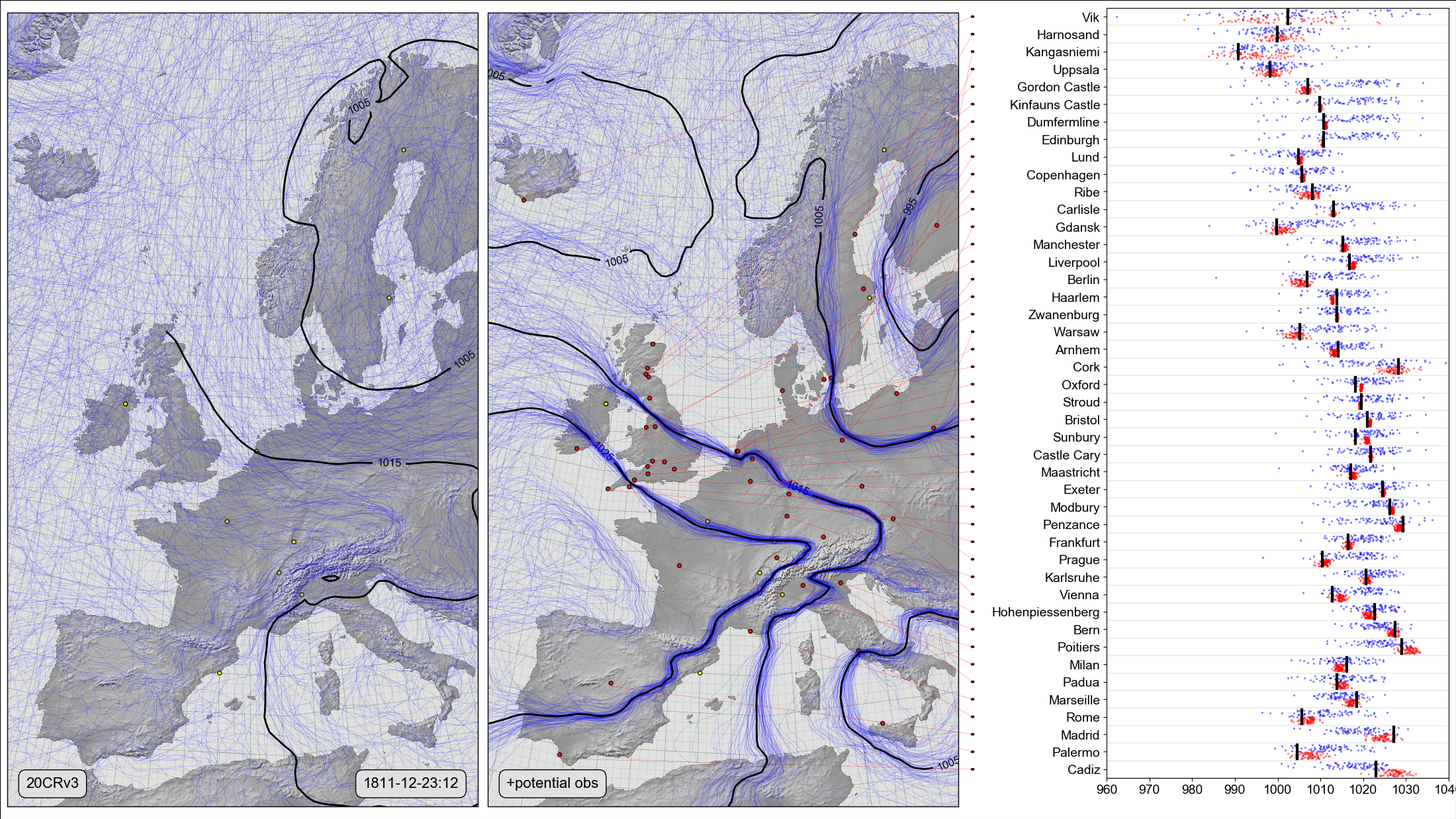
On the left, a Spaghetti-contour plot of 20CRv3 MSLP at noon on December 23rd 1811. Centre and right, Scatter-contour plot comparing the same field, after assimilating 44 fake observations at that date. The centre panel shows the 20CRv3 ensemble after assimilating all 44 fake observations (red dots). The right panel compares the two ensembles with the new observations: Black lines show the observed pressures, blue dots the original 20CRv3 ensemble at the station locations, and red dots the 20CR ensemble after assimilating all the observations except the observation at that location.
We know of 44 european stations making pressure observations in December 1811, but not available to 20CRv3 - these observations have not yet been rescued. To give some idea of how much the uncertainties in the reanalysis would reduce if these observations were available, we can assimilate a fake observation at each station. To make the fake observations, we took the mslp from ensemble member 1 of 20CRv3 at the location of each station, at the time of the field, and added a bit of noise (normaly distributed random with 1hPa standard deviation). Because the fake observations were all taken from the same ensemble member, they are mutually consistent, and can be collectively assimilated. But the resulting post-assimilation ensemble will be clustered around the ensemble member used, rather than the (unknown) real weather.
This weather map should give a reasonable estimate of the quality of reconstruction we could get if observations were rescued for all these stations, but it’s not an accurate map of the actual weather at the time.
Code to make the figure
Collect the reanalysis data (prmsl ensemble and observations from 20CRv3 for 1811):
#!/usr/bin/env python

import IRData.twcr as twcr
import datetime

dte=datetime.datetime(1905,3,1)
for version in (['4.5.1']):
    twcr.fetch('prmsl',dte,version=version)
    twcr.fetch_observations(dte,version=version)
Script to calculate a leave-one-out assimilation for one station:
#!/usr/bin/env python

# Make fake station observations for a set of locations
# Assimilate all but one station
#   and store the resulting field.

import os
import math
import datetime
import numpy
import pandas
import pickle

import iris
import iris.analysis

import IRData.twcr as twcr

import DIYA
import sklearn
RANDOM_SEED = 5

# Try and get round thread errors on spice
import dask
dask.config.set(scheduler='single-threaded')

obs_error=5 # Pa
model=sklearn.linear_model.Lasso(normalize=True)

opdir="%s/images/DWR_fake" % os.getenv('SCRATCH')
if not os.path.isdir(opdir):
    os.makedirs(opdir)

# Get the datetime, and station to omit, from commandline arguments
import argparse
parser = argparse.ArgumentParser()
parser.add_argument("--year", help="Year",
                    type=int,required=True)
parser.add_argument("--month", help="Integer month",
                    type=int,required=True)
parser.add_argument("--day", help="Day of month",
                    type=int,required=True)
parser.add_argument("--hour", help="Time of day (0,3,6,9,12,18,or 21)",
                    type=int,required=True)
parser.add_argument("--omit", help="Name of station to be left out",
                    default=None,
                    type=str,required=False)
args = parser.parse_args()

dte=datetime.datetime(args.year,args.month,args.day,
                      int(args.hour),int(args.hour%1*60))

# 20CRv3 data
prmsl=twcr.load('prmsl',dte,version='4.5.1')

# Fake the DWR observations for that time
obs=pandas.read_csv('stations.csv',header=None,
                    names=('name','latitude','longitude'))
obs=obs.assign(dtm=pandas.to_datetime(dte))
# Throw out the ones already used in 20CRv3
obs=obs[~obs['name'].isin(['Ylitornio','Paris','Turin','Geneva',
                           'Barcelona','Stockholm' ])]
# Also throw out the specified station
if args.omit is not None:
   obs=obs[~obs['name'].isin([args.omit])]
# Fill in the value for each ob from ens member 1
prmsl_r=prmsl.extract(iris.Constraint(member=1))
interpolator = iris.analysis.Linear().interpolator(prmsl_r,
                                   ['latitude', 'longitude'])
value=numpy.zeros(len(obs))
for i in range(len(obs)):
    value[i]=interpolator([obs.latitude.values[i],
                           obs.longitude.values[i]]).data
# Add some simulated obs error - 100hPa normal
value=value+numpy.random.normal(loc=0.0, scale=100.0, size=len(value))
obs['value'] = pandas.Series(value, index=obs.index)

# Update mslp by assimilating all obs.
prmsl2=DIYA.constrain_cube(prmsl,
                           lambda dte: twcr.load('prmsl',dte,version='4.5.1'),
                           obs=obs,
                           obs_error=obs_error,
                           random_state=RANDOM_SEED,
                           model=model,
                           lat_range=(20,85),
                           lon_range=(280,60))

dumpfile="%s/%04d%02d%02d%02d.pkl" % (opdir,args.year,args.month,
                                      args.day,args.hour)
if args.omit is not None:
    dumpfile="%s/%04d%02d%02d%02d_%s.pkl" % (opdir,args.year,args.month,
                                             args.day,args.hour,args.omit)

pickle.dump( prmsl2, open( dumpfile, "wb" ) )
Calculate the leave-one-out assimilations for all the stations: (This script produces a list of calculations which can be done in parallel):
#!/usr/bin/env python

# Do all the jacknife assimilations for a range of times

import os
import sys
import time
import subprocess
import datetime
import pandas

# Where to put the output files
opdir="%s/images/DWR_fake" % os.getenv('SCRATCH')
if not os.path.isdir(opdir):
    os.makedirs(opdir)

# Function to check if the job is already done for this time+omitted station
def is_done(dte,omit):
    opfile="%s/%04d%02d%02d%02d.pkl" % (opdir,dte.year,dte.month,
                                        dte.day,dte.hour)
    if omit is not None:
        opfile="%s/%04d%02d%02d%02d_%s.pkl" % (opdir,dte.year,dte.month,
                                               dte.day,dte.hour,omit)
    if os.path.isfile(opfile):
        return True
    return False

start_day=datetime.datetime(1811, 12, 23, 12)
end_day  =datetime.datetime(1811, 12, 23, 12)

f=open("run.txt","w+")

dte=start_day
while dte<=end_day:

    # Fake the stations for this point in time?
    obs=pandas.read_csv('stations.csv',header=None,
                        names=('name','latitude','longitude'))
    obs=obs.assign(dtm=pandas.to_datetime(dte))
    # Throw out the ones already used in 20CRv3
    obs=obs[~obs['name'].isin(['Ylitornio','Paris','Turin','Geneva',
                           'Barcelona','Stockholm'])]
    stations=obs.name.values.tolist()
    stations.append(None) # Also do case with all stations

    for station in stations:

        if is_done(dte,station): continue
        cmd="./leave-one-out.py --year=%d --month=%d --day=%d --hour=%d" % (
                  dte.year,dte.month,dte.day,dte.hour)
        if station is not None:
            cmd="%s --omit=%s" % (cmd,station)
        cmd="%s\n" % cmd
        f.write(cmd)
    dte=dte+datetime.timedelta(hours=6)
f.close()
Plot the figure:
#!/usr/bin/env python

# Assimilation of many stations.
# Plot the precalculated leave-one-out assimilation results

import os
import math
import datetime
import numpy
import pandas
import pickle
from collections import OrderedDict

import iris
import iris.analysis

import matplotlib
from matplotlib.backends.backend_agg import \
             FigureCanvasAgg as FigureCanvas
from matplotlib.figure import Figure
from matplotlib.patches import Circle

import cartopy
import cartopy.crs as ccrs

import Meteorographica as mg
import IRData.twcr as twcr


# Where are the precalculated fields?
ipdir="%s/images/DWR_fake" % os.getenv('SCRATCH')

# Date to show
year=1811
month=12
day=23
hour=12
dte=datetime.datetime(year,month,day,hour)

# Landscape page
aspect=16/9.0
fig=Figure(figsize=(22,22/aspect),  # Width, Height (inches)
           dpi=100,
           facecolor=(0.88,0.88,0.88,1),
           edgecolor=None,
           linewidth=0.0,
           frameon=False,
           subplotpars=None,
           tight_layout=None)
canvas=FigureCanvas(fig)
font = {'family' : 'sans-serif',
        'sans-serif' : 'Arial',
        'weight' : 'normal',
        'size'   : 14}
matplotlib.rc('font', **font)

# UK-centred projection
projection=ccrs.RotatedPole(pole_longitude=183.5, pole_latitude=35.5)
scale=20
extent=[scale*-1*aspect/3.0,scale*aspect/3.0,scale*-1,scale]

# On the left - spaghetti-contour plot of original 20CRv3
ax_left=fig.add_axes([0.005,0.01,0.323,0.98],projection=projection)
ax_left.set_axis_off()
ax_left.set_extent(extent, crs=projection)
ax_left.background_patch.set_facecolor((0.88,0.88,0.88,1))
mg.background.add_grid(ax_left)
land_img_left=ax_left.background_img(name='GreyT', resolution='low')

# 20CRv3 data
prmsl=twcr.load('prmsl',dte,version='4.5.1')

obs_t=twcr.load_observations_fortime(dte,version='4.5.1')
# Filter to those assimilated and near the UK
obs_s=obs_t.loc[((obs_t['Latitude']>0) &
                 (obs_t['Latitude']<90)) &
              ((obs_t['Longitude']>240) |
                 (obs_t['Longitude']<100))].copy()

# Plot the observations
mg.observations.plot(ax_left,obs_s,radius=0.1)

# PRMSL spaghetti plot
mg.pressure.plot(ax_left,prmsl,scale=0.01,type='spaghetti',
                   resolution=0.25,
                   levels=numpy.arange(875,1050,10),
                   colors='blue',
                   label=False,
                   linewidths=0.1)

# Add the ensemble mean - with labels
prmsl_m=prmsl.collapsed('member', iris.analysis.MEAN)
prmsl_s=prmsl.collapsed('member', iris.analysis.STD_DEV)
prmsl_m.data[numpy.where(prmsl_s.data>1000)]=numpy.nan
mg.pressure.plot(ax_left,prmsl_m,scale=0.01,
                   resolution=0.25,
                   levels=numpy.arange(875,1050,10),
                   colors='black',
                   label=True,
                   linewidths=2)

mg.utils.plot_label(ax_left,
              '20CRv3',
              fontsize=16,
              facecolor=fig.get_facecolor(),
              x_fraction=0.04,
              horizontalalignment='left')

mg.utils.plot_label(ax_left,
              '%04d-%02d-%02d:%02d' % (year,month,day,hour),
              fontsize=16,
              facecolor=fig.get_facecolor(),
              x_fraction=0.96,
              horizontalalignment='right')

# In the centre - spaghetti-contour plot of 20CRv3 with DWR assimilated
ax_centre=fig.add_axes([0.335,0.01,0.323,0.98],projection=projection)
ax_centre.set_axis_off()
ax_centre.set_extent(extent, crs=projection)
ax_centre.background_patch.set_facecolor((0.88,0.88,0.88,1))
mg.background.add_grid(ax_centre)
land_img_centre=ax_centre.background_img(name='GreyT', resolution='low')

# Fake the DWR observations for that afternoon
obs=pandas.read_csv('stations.csv',header=None,
                    names=('name','latitude','longitude'))
obs=obs.assign(dtm=pandas.to_datetime(dte))
# Throw out the ones already used in 20CRv3
obs=obs[~obs['name'].isin(['Ylitornio','Paris','Turin','Geneva',
                           'Barcelona','Stockholm'])]
# Fill in the value for each ob from ens member 1
prmsl_r=prmsl.extract(iris.Constraint(member=1))
interpolator = iris.analysis.Linear().interpolator(prmsl_r,
                                   ['latitude', 'longitude'])
value=numpy.zeros(len(obs))
for i in range(len(obs)):
    value[i]=interpolator([obs.latitude.values[i],
                           obs.longitude.values[i]]).data
obs['value'] = pandas.Series(value, index=obs.index)

# Load the all-stations-assimilated mslp
prmsl2=pickle.load( open( "%s/%04d%02d%02d%02d.pkl" %
                          (ipdir,dte.year,dte.month,
                                    dte.day,dte.hour), "rb" ) )

mg.observations.plot(ax_centre,obs_s,radius=0.1)
mg.observations.plot(ax_centre,obs,
                     radius=0.1,facecolor='red',
                     lat_label='latitude',
                     lon_label='longitude')

# PRMSL spaghetti plot
mg.pressure.plot(ax_centre,prmsl2,scale=0.01,type='spaghetti',
                   resolution=0.25,
                   levels=numpy.arange(875,1050,10),
                   colors='blue',
                   label=False,
                   linewidths=0.1)

# Add the ensemble mean - with labels
prmsl_m=prmsl2.collapsed('member', iris.analysis.MEAN)
prmsl_s=prmsl2.collapsed('member', iris.analysis.STD_DEV)
prmsl_m.data[numpy.where(prmsl_s.data>1000)]=numpy.nan
mg.pressure.plot(ax_centre,prmsl_m,scale=0.01,
                   resolution=0.25,
                   levels=numpy.arange(875,1050,10),
                   colors='black',
                   label=True,
                   linewidths=2)

mg.utils.plot_label(ax_centre,
              '+potential obs',
              fontsize=16,
              facecolor=fig.get_facecolor(),
              x_fraction=0.04,
              horizontalalignment='left')


# Validation scatterplot on the right
obs=obs.sort_values(by='latitude',ascending=True)
stations=list(OrderedDict.fromkeys(obs.name.values))

ax_right=fig.add_axes([0.76,0.05,0.235,0.94])
# x-axis
xrange=[960,1040]
ax_right.set_xlim(xrange)
ax_right.set_xlabel('')

def pretty_name(name):
   return name.replace('_',' ')

# y-axis
ax_right.set_ylim([1,len(stations)+1])
y_locations=[x+0.5 for x in range(1,len(stations)+1)]
ax_right.yaxis.set_major_locator(
              matplotlib.ticker.FixedLocator(y_locations))
ax_right.yaxis.set_major_formatter(
              matplotlib.ticker.FixedFormatter(
                  [pretty_name(s) for s in stations]))

# Custom grid spacing
for y in range(0,len(stations)):
    ax_right.add_line(matplotlib.lines.Line2D(
            xdata=xrange,
            ydata=(y+1,y+1),
            linestyle='solid',
            linewidth=0.2,
            color=(0.5,0.5,0.5,1),
            zorder=0))

# Plot the station pressures
for y in range(0,len(stations)):
    station=stations[y]
    try:
        mslp=float(obs[obs.name==station].value/100.0)
    except KeyError: continue
    if mslp is None: continue
    ax_right.add_line(matplotlib.lines.Line2D(
            xdata=(mslp,mslp), ydata=(y+1.1,y+1.9),
            linestyle='solid',
            linewidth=3,
            color=(0,0,0,1),
            zorder=1))

# for each station, plot the reanalysis ensemble at that station
interpolator = iris.analysis.Linear().interpolator(prmsl,
                                   ['latitude', 'longitude'])
for y in range(len(stations)):
    station=stations[y]
    ensemble=interpolator([obs.latitude.values[y],
                           obs.longitude.values[y]])

    ax_right.scatter(ensemble.data/100.0,
                numpy.linspace(y+1.5,y+1.9,
                              num=len(ensemble.data)),
                20,
                'blue', # Color
                marker='.',
                edgecolors='face',
                linewidths=0.0,
                alpha=0.5,
                zorder=0.5)

# For each station, assimilate all but that station,
#     and plot the resulting ensemble
for y in range(len(stations)):
    station=stations[y]
    prmsl2=pickle.load( open( "%s/%04d%02d%02d%02d_%s.pkl" %
                                   (ipdir,dte.year,dte.month,
                                    dte.day,dte.hour,station), "rb" ) )
    interpolator = iris.analysis.Linear().interpolator(prmsl2,
                                   ['latitude', 'longitude'])
    ensemble=interpolator([obs.latitude.values[y],
                           obs.longitude.values[y]])
    ax_right.scatter(ensemble.data/100.0,
                numpy.linspace(y+1.1,y+1.5,
                              num=len(ensemble.data)),
                20,
                'red', # Color
                marker='.',
                edgecolors='face',
                linewidths=0.0,
                alpha=0.5,
                zorder=0.5)

# Join each station name to its location on the map
# Need another axes, filling the whole fig
ax_full=fig.add_axes([0,0,1,1])
ax_full.patch.set_alpha(0.0)  # Transparent background

def pos_left(idx):
    station=stations[idx]
    rp=ax_centre.projection.transform_points(ccrs.PlateCarree(),
                              numpy.asarray(obs.longitude.values[idx]),
                              numpy.asarray(obs.latitude.values[idx]))
    new_lon=rp[:,0]
    new_lat=rp[:,1]

    result={}
    result['x']=0.335+0.323*(new_lon-(scale*-1)*aspect/3.0)/(scale*2*aspect/3.0)
    result['y']=0.01+0.98*(new_lat-(scale*-1))/(scale*2)
    return result

# Label location of a station in ax_full coordinates
def pos_right(idx):
    result={}
    result['x']=0.668
    result['y']=0.05+(0.94/len(stations))*(idx+0.5)
    return result

for i in range(len(stations)):
    p_left=pos_left(i)
    if p_left['x']<0.335 or p_left['x']>(0.335+0.323): continue
    if p_left['y']<0.005 or p_left['y']>(0.005+0.94): continue
    p_right=pos_right(i)
    ax_full.add_patch(Circle((p_right['x'],
                              p_right['y']),
                             radius=0.001,
                             facecolor=(1,0,0,1),
                             edgecolor=(0,0,0,1),
                             alpha=1,
                             zorder=1))
    ax_full.add_line(matplotlib.lines.Line2D(
            xdata=(p_left['x'],p_right['x']),
            ydata=(p_left['y'],p_right['y']),
            linestyle='solid',
            linewidth=0.2,
            color=(1,0,0,1.0),
            zorder=1))

# Output as png
fig.savefig('Leave_one_out_%04d%02d%02d%02d.png' %
                                  (year,month,day,hour))