A DIY Machine Learning Climate Model

This is an example of how to build a climate model using Machine Learning (ML). It’s designed to be used as a training tool for those new to ML, but to be powerful enough to be adapted into something of value for science work.

The fundamental objective is to build a model that is useful for climate science - in particular, in this case, to predict and attribute changes in precipitation - but using ML, rather than a traditional physical model. A great virtue of this approach is the ML model is dramatically cheaper than a physical model, both to create and to use.

Background

Climate Scientists are mostly used to using physical models (GCMs). It is important to understand that ML models are quite a different thing - don’t think of an ML model as a new variant of GCM.

• When building a GCM we specify how the model behaves. The aim is to make the model as close to physical reality as possible. The results produced by the model are then an emergent property, and they will be correct if the model is an adequate representation of the real world. So, with a GCM, the focus is on the model itself.

• When building an ML model, we specify what the model learns. The aim is to make the model as good as possible at predicting the data we have given it. The results produced by the model are then a prediction, and they will be correct if the model has learned the patterns in the data. So, with an ML model, the focus is on the data used in training, and the model is an emergent property - ML models do have to correspond to reality, but they don’t have to do so in any way we’d recognize as physics.

So physical modellers care primarily about the physical correctness of their model, and only secondarily about their validation statistics. ML modellers care primarily about their validation statistics, and the issue of physical correctness does not arise. (Of course this is a simplification - real science is much more complex than this, but it is nonetheless an important distinction.)

A result of this is that GCMs are, in a sense, all trying to do the same thing - they are all trying to represent the same set of physical equations. ML models can be much more diverse - each is trying to predict its training data, and the training data can be anything. So GCMs are generic: one GCM - many applications. ML models are specific: we should expect to train a new model for each new problem. (It is possible to train generic ML models, but this is difficult, expensive, and will be less accurate than training a specific model. The majority of ML models used in climate will be problem-specific)

So the first task is to choose a problem. This model is built to study monthly precipitation - in particular to represent the spatial distribution of precipitation (to what extent can we infer the precipitation in London given the precipitation in Birmingham), and the relationship between precipitation and other variables (how does precipitation relate to 2m-air temperature and mean-sea-level pressure). This is a convenient example problem, but note that the model may well be of interest even if you don’t care about precipitation: The model we are training here is precipitation-specific, but the model code and structure are much more generic - you could take the same model specification, and the same software, and train it on a different dataset, to make an ML model of use for your own work.

Design Decisions

Our aim, with a climate model, is typically to generate an estimate of some future climate state, so the obvious tool is a generative model. That is, a model that will make new, plausible climate states.

Illustration of a generative model outputting a climate state.

So how do we make such a model? A principal virtue of ML, is that there are already several well established ML methods for making generative models, here we will use a Variational AutoEncoder (VAE). The VAE is a generative model factory - it learns such models from example inputs. The main virtue of the VAE is that it provides a specifically-constrained model state vector, which offers additional ways to control the model output, effectively allowing us to do data assimilation.

Illustration of a VAE - a factory for making generative models given examples of the desired output.

• Detailed specification of the ML model

Training data

To learn the model, we need good quality training data. We are modelling the relationships between 2m temperature, mean-sea-level-pressure, and precipitation, so we need training data for these three variables. We will get these data from the ERA5 reanalysis.

• How to download the training data

That provides the data, in original units (degrees Kelvin, pascals, and mm/s) as a collection of netCDF files. To use the data in an ML model, we need to make several transformations:

1. Regrid to a standard grid (not strictly necessary if we are only using ERA5 output, but I regrid it anyway to move the longitude range from 0-360 to -180-180 - let’s have the UK in the middle of the map).

2. Convert the data from netCDF to an efficient format for ML (I use serialized tf.tensors).

3. Normalize the data to be approximately normally distributed on the range 0-1 (I use quantile mapping).

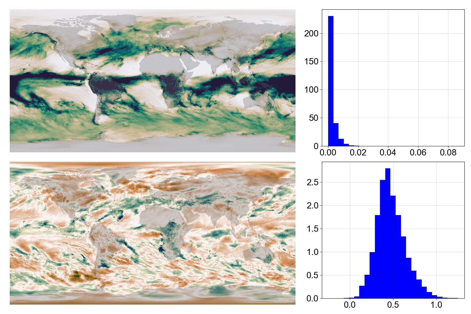
Precipitation (map and PDF) for March 1969. Raw data above, normalized data below.

• How to convert and normalize the data

Training the model

Once we have the data in the right format, we can train the model. The details are in the ML model specification. The key steps are:

• Specify the details of the model
• Assemble the normalized data into training and test datasets
• Train the model

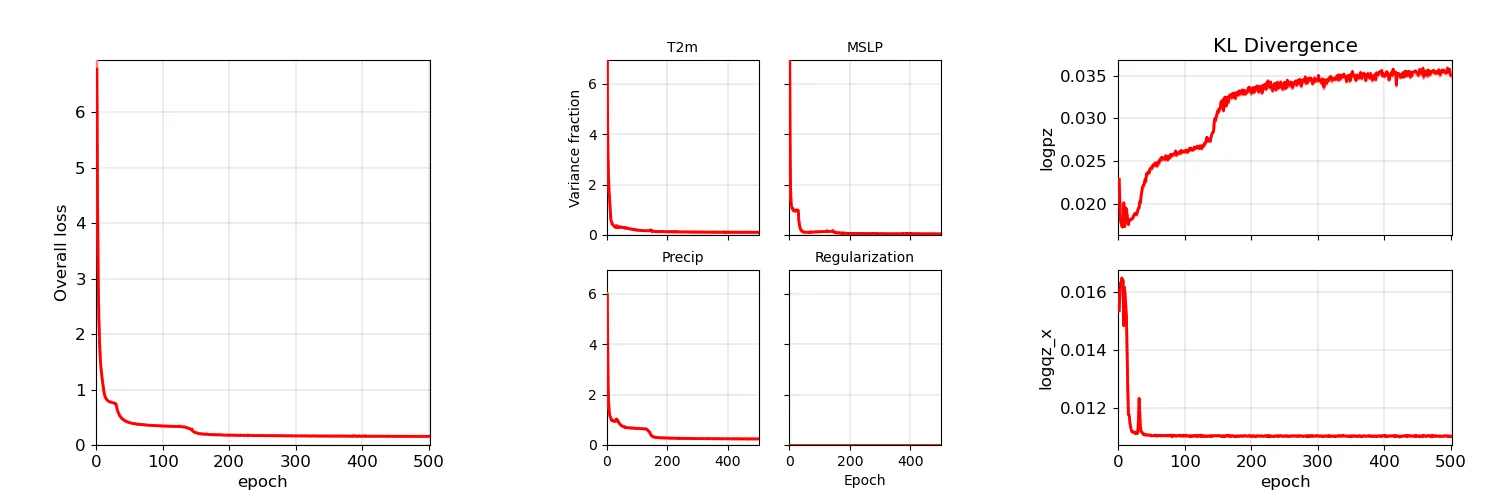
Model training progress plot. (More details)

We want to see the loss function get down close to zero, for both the training data (pale lines), and for the test data (darker lines). If the individual variable values are below one, then the model has skill - it’s better than climatology.

Validating the trained model

Once we have trained the model, we need to validate it. This is a crucial step - the model is only useful if it can predict data it has not seen before. We already know if the model has skill - we can see that from the training loss, but it’s worth looking in more detail:

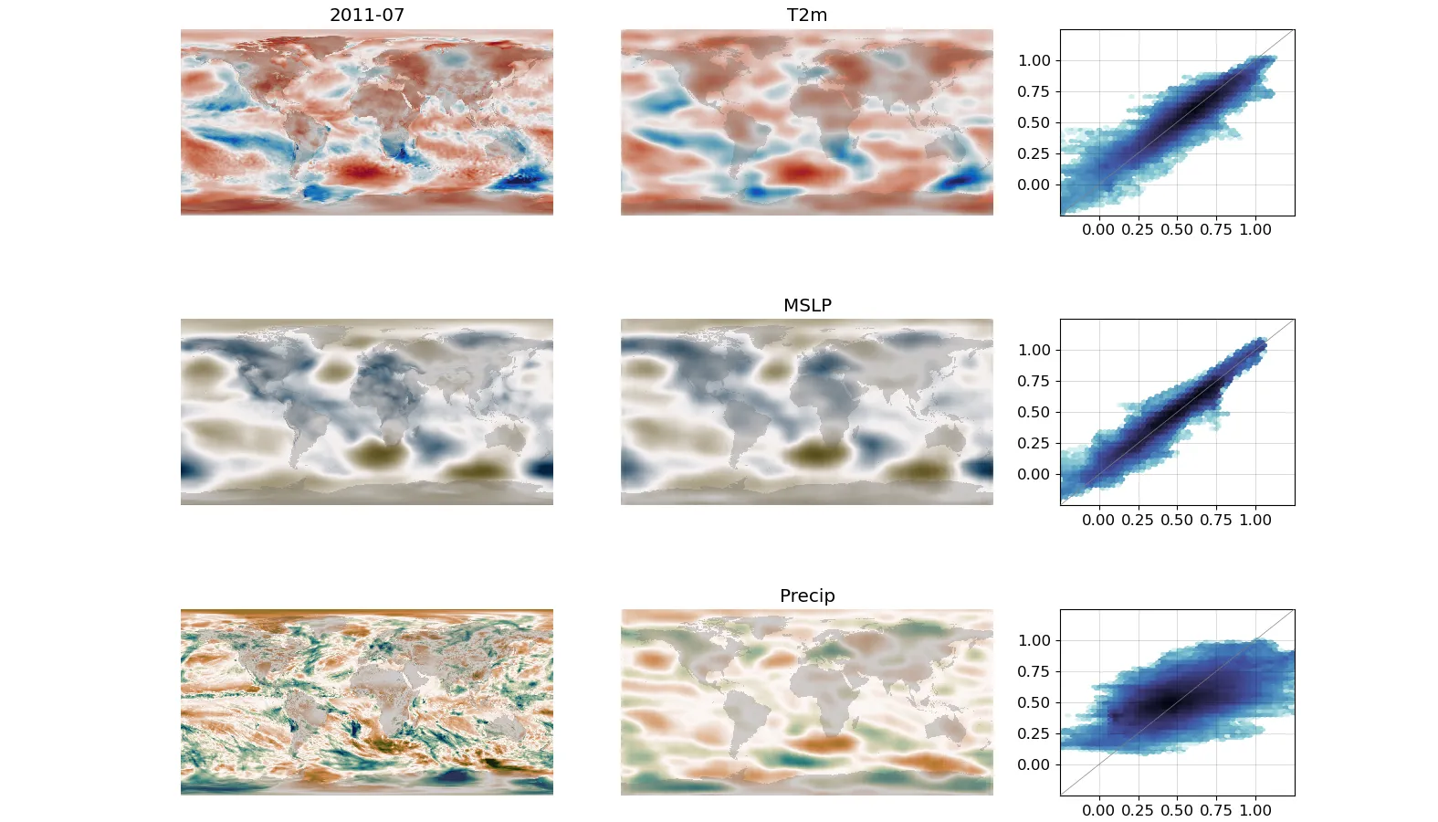
Model validation for a single month: Target on the left, model output in the middle, scatter comparison on the right. (More details)

And as well as looking at individual months, we can look at the model’s performance over the whole dataset:

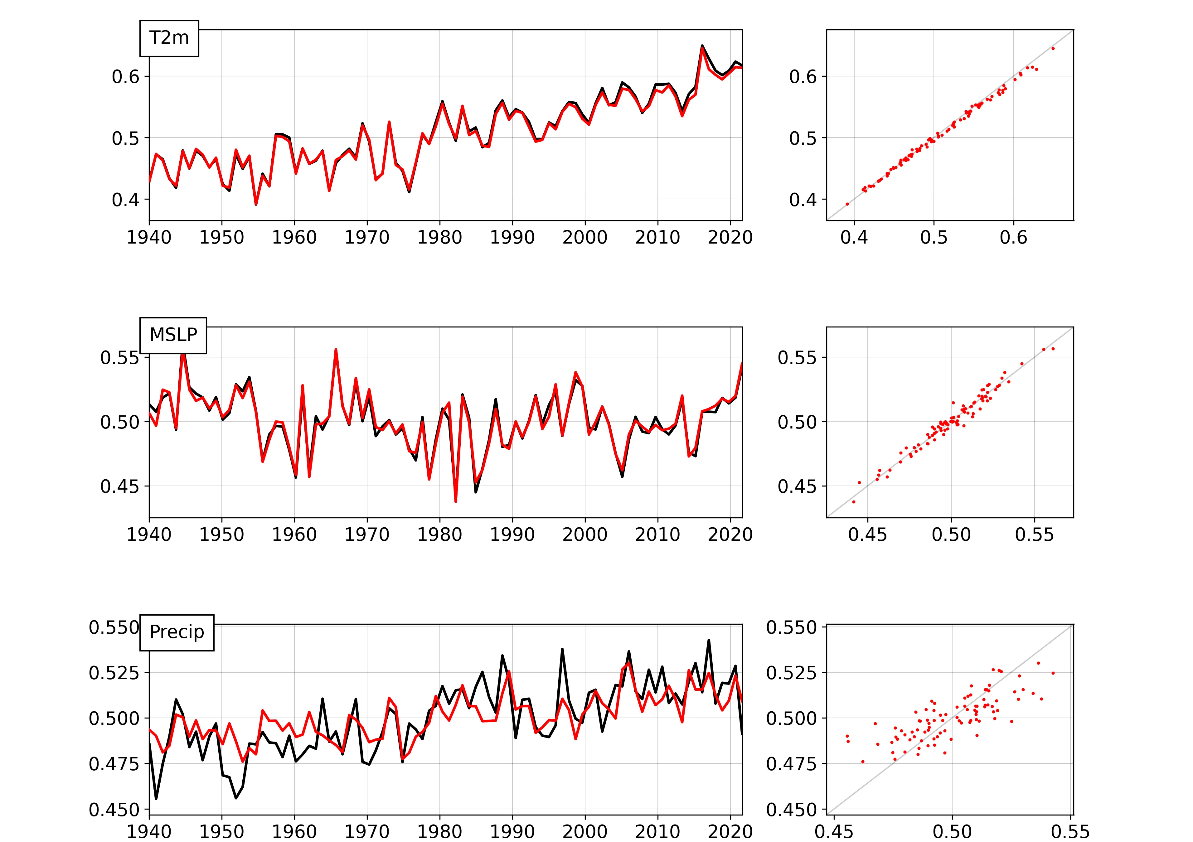
Model validation time-series: Global-mean values for each month in the test dataset - target in black, model output in red. (More details)

Clearly the VAE works usefully - good accuracy for T2m and MSLP, and reasonable accuracy for precipitation. The model is not perfect, but it is a useful tool for understanding the relationships between these variables.

Using as a generative model

So the DCVAE works well - it can convert fields of T2m and MSLP into an embedding, and then convert that embedding back into fields of T2m, MSLP, and Precip. But we want a generative model - to make new fields of T2m, MSLP, and Precip. To test this we just take the decoder half of the model, and generate the output fields from a random embedding.

To do this we use the assimilation scripts but don’t assimilate anything - just generate the fields from a random embedding.

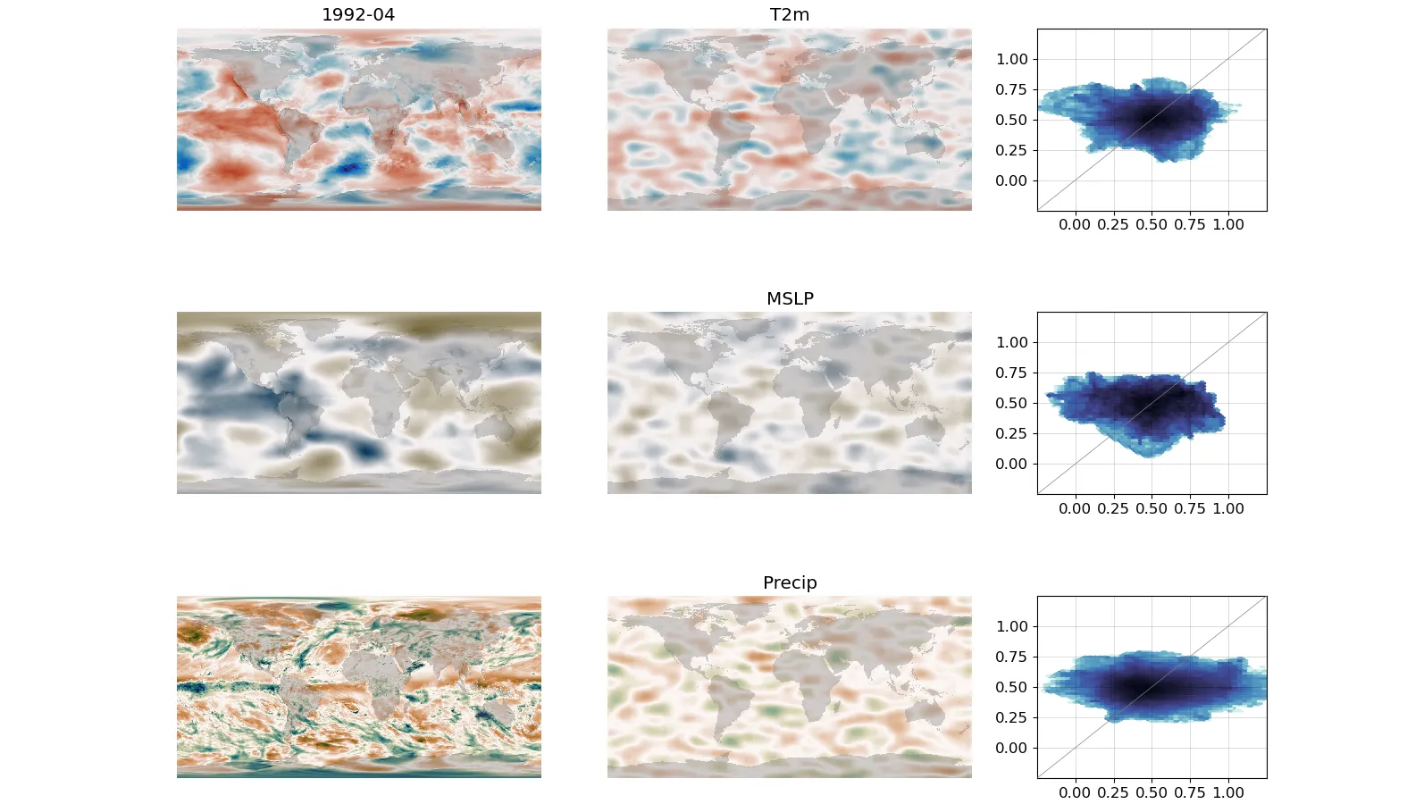
Left-hand column - a sample field from the test dataset. Centre column - a field generated from a random embedding. (Note that these columns should not be the same, but the centre column should look like the same sort of thing as the left-hand column). (More details)

It’s hard to say exactly how well this works - the model generated fields are not the same as the test dataset fields, but they are similar.

But the value of the method is not in unconstrained generation, but in constrained generation. We can do the same, but assimilating T2m and MSLP:

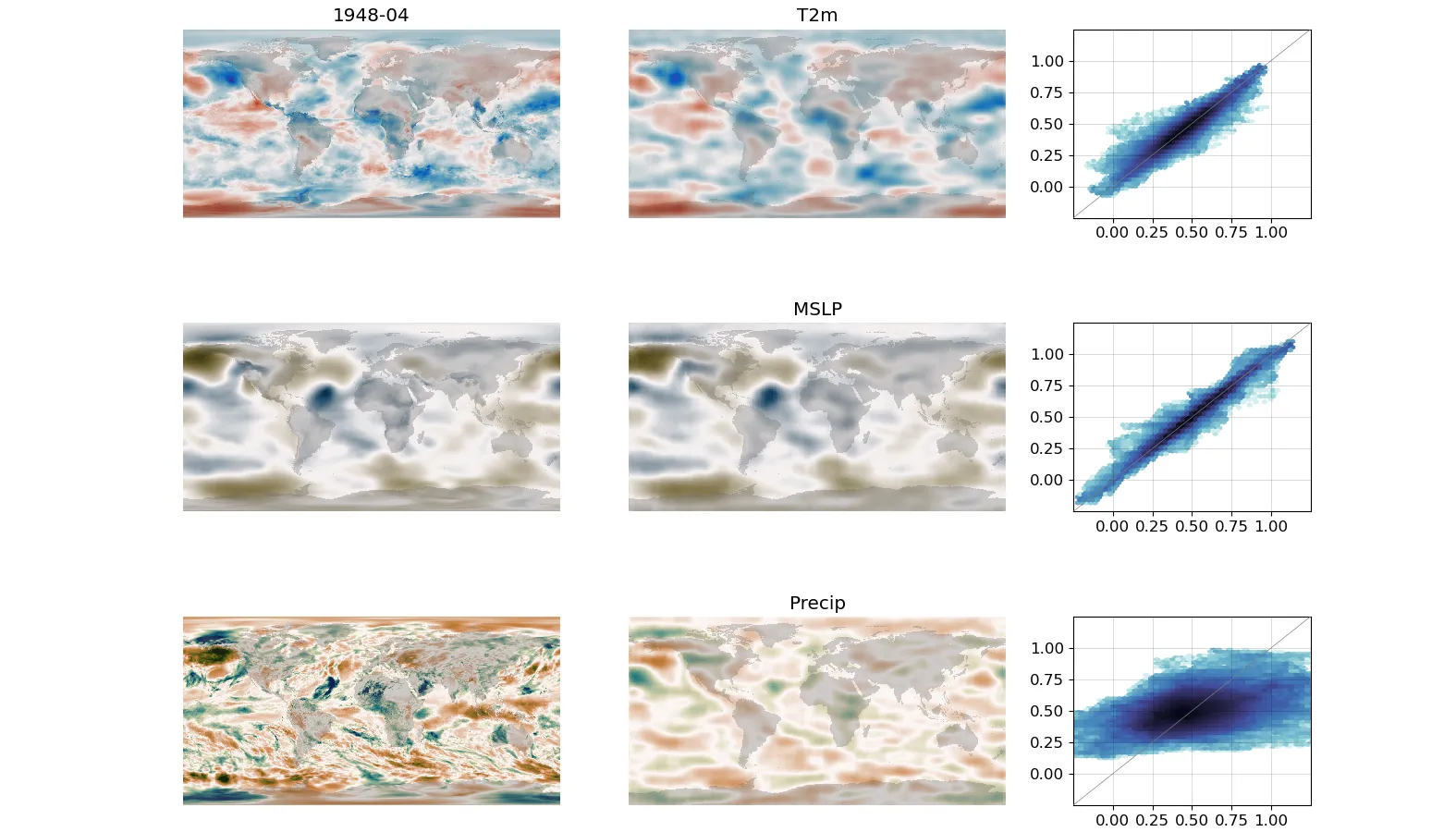
Left-hand column - a sample field from the test dataset. Centre column - a field generated from an embedding chosen to match the T2m and MSLP. (Precip is calculated by the model). (More details)

And if we make the time-series diagnostic the same way, we can see the point of the model:

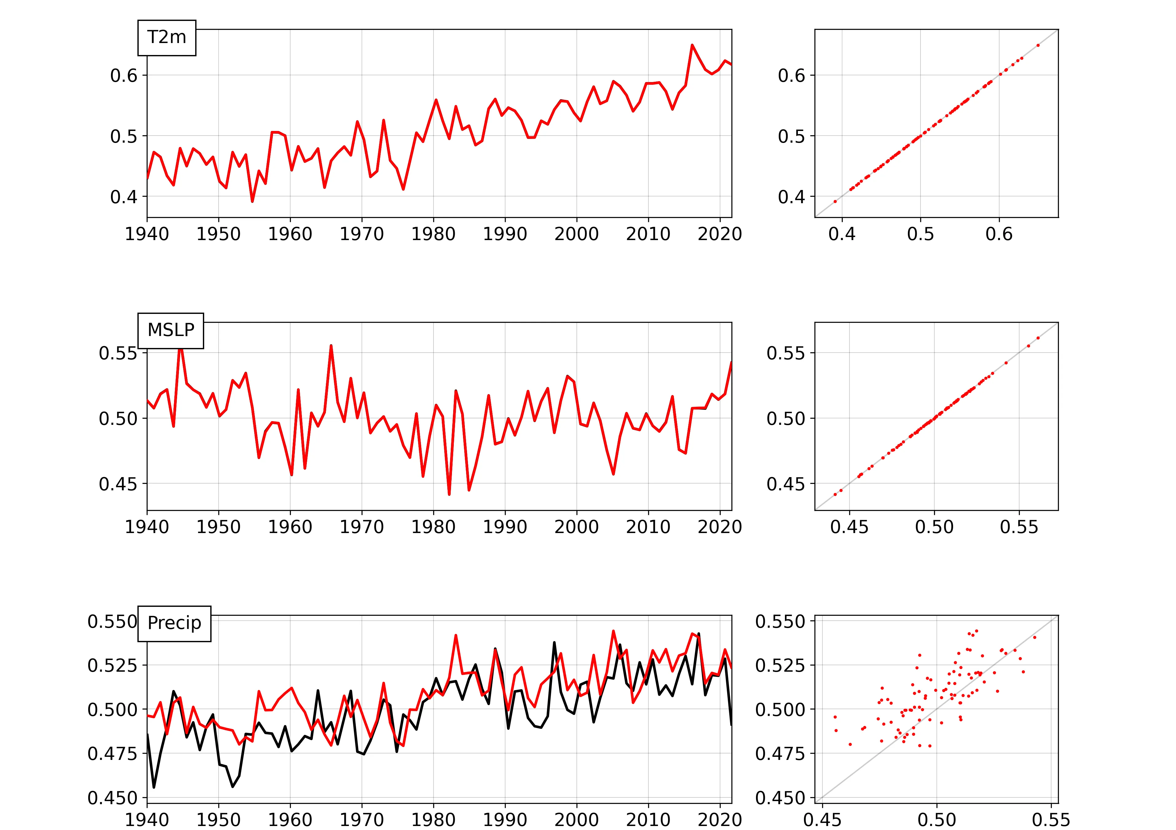
Global-mean values for each month in the test dataset - ERA5 data in black, model output in red. Here T2m and MSLP have been assimilated, Precip is calculated by the model. (More details)

We can now compare observed (ERA5) and modelled precipitation, where the modelled precipitation is calculated from observed T2m and MSLP. We can see a notable divergence between the ERA5 and modelled precipitation before about 1980 - this demonstrates the biases in the ERA5 precipitation product.

And we can go on to do an attribution study: Does the trend in precip have a common origin with the trend in T2m? We can test this by only assimilating MSLP - don’t force the T2m trend - and seeing what the calculated Precip does.

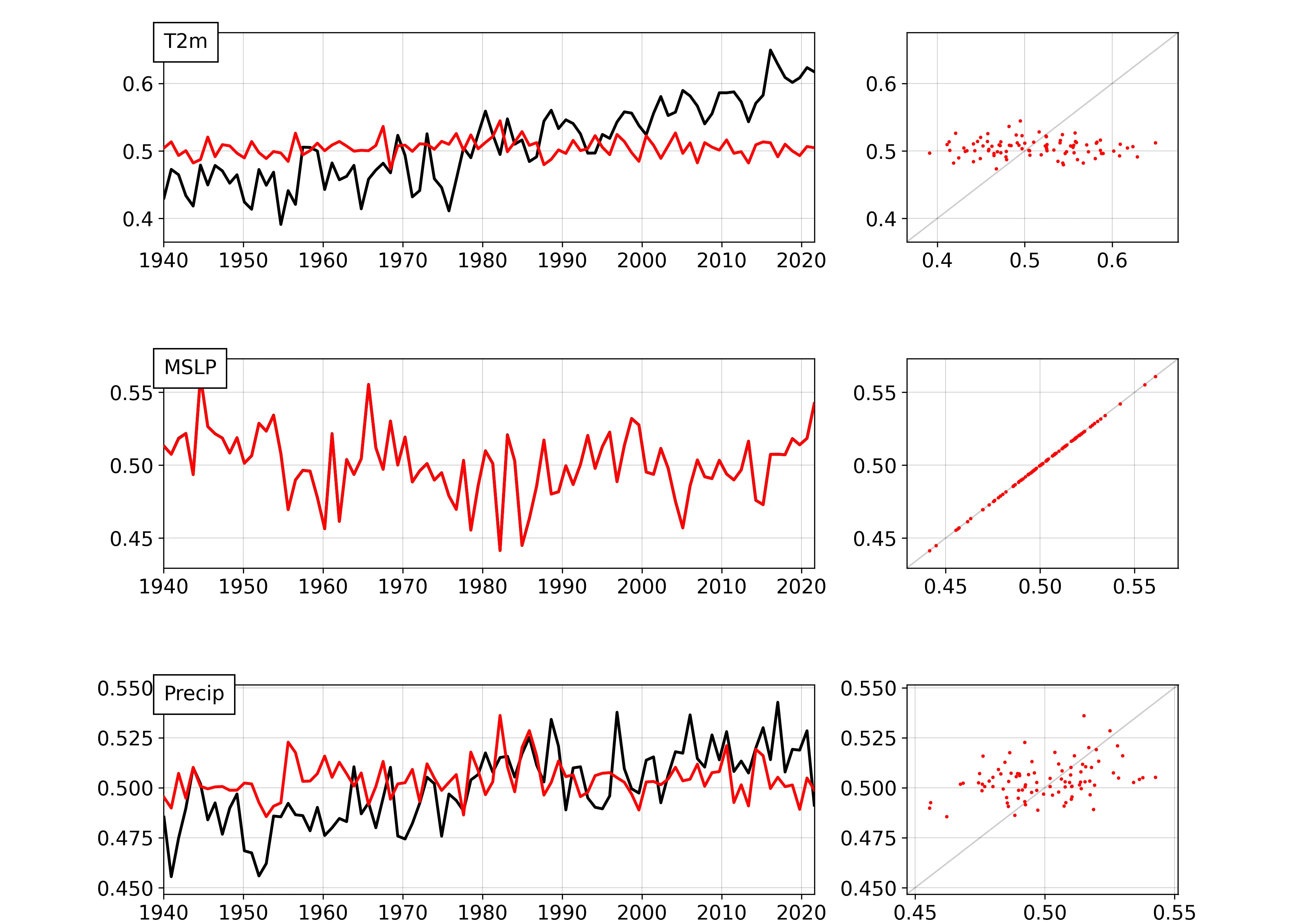
Global-mean values for each month in the test dataset - ERA5 data in black, model output in red. MSLP has been assimilated, T2m and Precip are calculated by the model. (More details)

The model is now answering the question ‘What would the global Precip trend have looked like if there were no temperature trend?’ And the answer is clear - the Precip trend is driven by the T2m trend - or at least by a common factor (the CO2 increase).

Conclusions

If we want to understand, predict, and attribute climate change, we don’t need a GCM. We can use ML (and specifically the DCVAE) to build an alternative model, and then use the ML model to answer the questions we have.

Next steps

This model is trained on monthly T2m, MSLP and Precip. But we could use the same model design on other variables, or at other time-scales. It’s just a matter of getting the data, normalizing it, and training the model. What else can we investigate the same way?

The model is pretty good, but it could be better. Can we improve the model design, or find better hyperparameters?

Go on - try it yourself.

Appendices

• Utility functions for plotting and regridding

Small print

• How to reproduce or extend this work
• Authors and acknowledgements

This document is crown copyright (2024). It is published under the terms of the Open Government Licence. Source code included is published under the terms of the BSD licence.